Introduction
Pseudo-stereophony audio processing techniques generate two stereo channels from a single mono one, in order to generate a wider spatial impression. The need for pseudo-stereo techniques arose with the development of commercial stereo reproduction and distribution, to attempt to bring existing mono audio material into the new medium. Nonetheless, pseudo-stereo can also be used as a creative audio manipulation tool in itself. It is important to note that pseudo-stereo techniques are also sometimes called pseudo-stereo synthesizers precisely because they artificially create the spatial information. Even though stereo width manipulation using Mid-Side balancing (starting with a Mid (L+R) signal and adding/subtracting varying amounts of Side (L-R) signal to increase width) is sometimes referred to in literature as pseudo-stereo, it is not a pseudo-stereo technique, because it uses spatial characteristics–in the form of phase difference–already present in the original stereo signals.
Pseudo-stereo has been explored in two different scenarios: loudspeaker and headphone reproduction. The type of reproduction will significantly affect the result of the process, because using loudspeakers, both ears are getting the signal from both speakers, producing comb filtering, while headphone reproduction has isolation between the signals, but does not provide HRTF cues and is free from room reverberation. So the perceived effect of pseudostereo techniques will be different for loudspeaker and headphone listening. Pseudo-stereophony techniques tend to have a bad reputation in audio engineering circles because although they significantly enhance spatial perception, they produce unacceptable side effects like phasiness, a sound that is tiring to listen to or unacceptable degradation of the sound.
Pseudo-stereo in practice
The exact approach and effect of pseudo-stereo techniques has always been somewhat vague. While some authors have developed pseudo-stereo techniques in an attempt to increase the perceived width of the audio source, others have attempted to achieve different spatial locations for different spectromorphologically related elements of the audio source. So, even though some authors seek either image spread or image separation, in practice, you will tend to have both with complex audio material, with hard to predict and inconsistent results. For this reason, usage of pseudo-stereo algorithms requires careful attention to detail and fine tuning to achieve results that will not be regretted down the road.
It is understood that differences between the sound at each ear are interpreted as spatial information. These differences are usually characterized using the Inter-Aural Cross-correlation Coefficient (IACC), which is the maximum absolute peak of the cross-correlation between both signals. Pseudo-stereo techniques produce perception of space precisely because they generate slight differences between the signals at each ear which the brain interprets as spatial cues.
I. Time Delay between speakers
The simplest pseudo-stereo technique consists of adding a small delay to a signal. Lauridsen experimented with this technique [1], reproducing it not over a conventional stereo system, but on a pair of speakers radiating at a 90° angle, using delays between 50ms and 150ms as shown in Figure 1. The farther speaker, which points to the side, was used unbaffled, so it can project a wavefront &ndash inverted in phase with relation to its front&ndash on its rear.
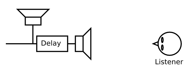
If the playback occurs in free-field conditions, e.g. an anechoic chamber, and the speakers have ideal directivity characteristics, one ear of the listener would receive the far speaker in phase, while the other side would receive it in anti-phase. This signal from the far speaker would add to the signal from the delayed near speaker, to produce comb filtering. Thus, since both channels effectively have different frequency responses, each channel's signals are different, and this will produce IACC differences. This effect is in fact enhanced since the room provides further decorrelation through reverb and irregularities in speaker directivity.
Though this technique may be useful to counter the precedence effect, its results are location dependent, as a delay that works well for a certain location will not work for another. It is also source-material dependent as some delay times will colour certain material in unacceptable ways, while being suitable for others.
II. Complementary filters
Complementary Comb Filters
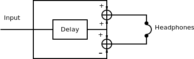
The natural extension to the previous technique was also proposed by Lauridsen. Instead of having the signals from both loudspeakers added in the air when reaching the ear, he proposed adding them electronically for headphone reproduction, as shown in Figure 2. Adding a signal to a delayed version of itself is in effect a comb filter. By adding the signals electornically, what happens is that a pair of complementary comb filters is realized. This means that a dip in one channel matches a peak in the other. The system can have control of the size and number of filter bands by adjusting the delay time.
Below is an implementation of the Lauridsen technique of complementary comb filters:
opcode lauridsen, aa, ak
	ain, kdelay xin

	imaxdel = 30
	kdelay limit kdelay, 0.001, imaxdel
	adelay1 vdelay3 ain, kdelay, imaxdel
	aleft = -ain + adelay1
	aright = ain + adelay1

	xout aleft*0.5, aright*0.5
endop
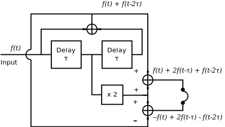
Schroeder studied the factors that play a greatest role in spatial impression in these types of complementary filters for headphone reproduction [2]. He showed that it was the intensity variations in frequency rather than the phase differences between each channel that had the greatest effect. Taking advantage of this he designed a set of complementary comb filters, as shown in Figure 3, which produce the same phase response on both channels. This system can have control of the size and number of filter bands by adjusting the delay time.
Below is shown an implementation of the Schroeder complemenary comb filters as a Csound UDO:
opcode schroeder, aa, ak
	ain, kdelay xin

	imaxdel = 30
	kdelay limit kdelay, 0.001, imaxdel
	adelay1 vdelay3 ain, kdelay, imaxdel
	adelay2 vdelay3 adelay1, kdelay, imaxdel
	aleft = -ain + (2 * adelay1) - adelay2
	aright = ain + (2 * adelay1) + adelay2

	xout aleft*0.5, aright*0.5
endop
There are two significant issues with these techniques, which are also the reason why these techniques are not favoured by critical listeners. They both produce strong coloration: the signal sounds noticeably different from the original, and phasiness is present due to the sharp comb filters. Consequently, they are rarely used nowadays. Although their effect is quite dramatic and noticeable it is also tiring to listen to after a while.
All-pass networks
Bauer proposed the usage of all-pass networks to produce phase difference between two channels [3]. He proposed this technique for loudspeaker reproduction, so his reports that spatial impression was notably affected does not seem to contradict Schroeder's findings for headphones, as there will be filtering in the amplitude through the addition in the air of both signals. He does note however that more reverberant rooms tend to lessen the effect.
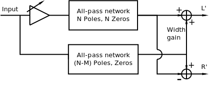
Orban proposed an enhancement to this technique that adds the all-pass networks, and through a gain control allows controlling the amount of image spread [4]. His method is shown in Figure 4. Orban suggests setting N = 4 and M= 2,3,4.
An all-pass filter can be produced in Csound using the following UDO:
opcode AllPass, a, a
	ain xin
	; Generate stable poles
	irad exprand 0.1
	irad = 0.99 - irad
	irad limit irad, 0, 0.99
	;iang random -$M_PI, $M_PI
	iang random -$M_PI, $M_PI
	ireal = irad * cos(iang)
	iimag = irad * sin(iang)
	print irad, iang, ireal, iimag

	; Generate coefficients from poles
	ia2 = (ireal * ireal) + (iimag * iimag)
	ia1 = -2*ireal
	ia0 = 1

	ib0 = ia2
	ib1 = ia1
	ib2 = ia0

	printf_i "ia0 = %.8f ia1 = %.8f ia2= %.8f\n", 1, ia0, ia1, ia2
	aout biquad ain, ib0, ib1, ib2, ia0, ia1, ia2

	xout aout
endop
This UDO produces the filter coefficients for an IIR biquad filter by randomly generating stable poles which guarantee an all-pass response. This UDO in particular produces a 2-pole all-pass filter.
This UDO can then be used to realize the Orban method like below (including selection of number of poles for the second filter):
opcode Orban, aa, akk
	ain, kwidth, kmode xin
	;; Cascade two filters to create a 4-pole all-pass
	a1 AllPass ain
	a1 AllPass a1

	a2 AllPass ain
	if kmode == 1 then
		a2 AllPass a2
	endif

	aout1 = a1*kwidth + a2
	aout2 = - a1*kwidth + a2

	xout aout1, aout2
endop
It is important to note that since the filter coefficients are random, there are infinitely many different filters which could be used in combination. Usually, the best combination must be determined by trial and error as different filters will have different effects on different material.
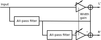
Gerzon proposed a further refinement which allows very precise control over the characteristics of the complementary filters [5]. It uses two identical all-pass filters, as the basis for construction of comb filters. It is shown in Figure 5. Like the Orban method, the spread can be controlled using gain on one of the paths to each channel. It must be noted that this method is no longer completely mono-compatible, although it can have less artifacts than the previous one.
The method can be realized in Csound using a UDO below, which has a mode parameter to select the number of poles of the all-pass filters by chaining two-pole all-pass filters:
opcode Gerzon, aa, akk
	ain, kwidth,kmode xin
	a1 AllPass ain
	a2 AllPass a1

	if kmode > 0 then
		a1 AllPass a1
		a2 AllPass a1
	endif
	if kmode > 1 then
		a1 AllPass a1
		a2 AllPass a1
	endif
	if kmode > 2 then
		a1 AllPass a1
		a2 AllPass a1
	endif
	if kmode > 3 then
		a1 AllPass a1
		a2 AllPass a1
	endif
	if kmode > 4 then
		a1 AllPass a1
		a2 AllPass a1
	endif
	if kmode > 5 then
		a1 AllPass a1
		a2 AllPass a1
	endif
	if kmode > 6 then
		a1 AllPass a1
		a2 AllPass a1
	endif

	aout1 = ain*kwidth + a1
	aout2 = -a2*kwidth + a1

	xout aout1, aout2
endop
Gerzon mentions that one of the purposes of this technique is to do "simulation of the size of a sound source" [5]. Both Schroeder and Gerzon envisioned this process as one that could also be applied individually to individual mono components of a stereo mix.
In essence as Gauthier states [6], any combination of inverted filtering can serve as pseudo-stereo filters for artistic purposes. This could be done both with time domain filtering or with frequency domain filtering.
III. Frequency modulation
Artificial Double Tracking (ADT) is a recording technique developed to generate a second channel of lead vocal from one take, using a second synchronized tape machine. The second machine would have small delay and a amount of wow and flutter effectively modulating the signal. The original signal is sent to one channel, while the second signal goes to the other. The variations in frequency between both signals will create a modulated comb filter, which in turn produces variations in IACC, perceived as spatial properties if the modulation is small enough. The wow and flutter can be modeled as simple periodical modulation, or using some form of interpolated jitter:
opcode modulate, a, akkkki
	ain, kfreq, kamp, ktype, kdelay, imaxtime xin
	if ktype == 0 then
		amod jspline kamp, kfreq, kfreq
	elseif ktype == 1 then
		amod poscil kamp, kfreq, 1
	elseif ktype == 2 then
		amod poscil kamp, kfreq, 2
	endif

	aout vdelay3 ain, kdelay *(1.00001 + amod), imaxtime
	xout aout
endop
The processing would then look like:
	aflutter modulate gainput, gkflutter_freq, gkflutter_amt, gkflutter_type, gkdelay_adt, 100
	awow modulate aflutter, gkwow_freq, gkwow_amt, gkwow_type, gkdelay_adt, 100
	aout1 = gainput*gklevel_adt
	aout2 = awow*gklevel_adt
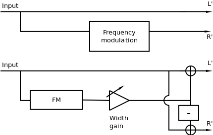
A variation of this technique, implemented by hbasm's Stereoizer plugin, adds phase inverted chorus to the dry signal on each channel. Mono downmix will result in the original signal, while chorusing will be heard on each individual channel. These techniques are pictured in Figure 6.
	aflutter modulate gainput, gkflutter_freq, gkflutter_amt, gkflutter_type, gkdelay_adt, 100

	aout1 = (gainput + (aflutter*gkwidth_adt) )*gklevel_adt
	aout2 = (gainput - (aflutter*gkwidth_adt) )*gklevel_adt
IV. Artificial decorrelation
Artificial decorrelation is defined by Kendall as the "process whereby an audio source signal is transformed into multiple output signals with waveforms that appear different to each other but which sound the same as the source" [7]. In the same article, Kendall proposes a method to spread a monophonic source over multiple loudspeakers using artificial decorrelation. Kendall proposed using FIR filters derived from doing inverse FFT from a spectrum which is flat, but with phases randomized between +Π and -Π. Additionally, the amount of decorrelation can be controlled by mixing the phase vectors before doing the IFFT to decrease the decorrelation. Alternatively, instead of designing a filter this way, a set of coefficients which can provide decorrelation can be obtained from MLS (Maximal length sequences) or Golay codes sequences.
In this technique there is a trade-off between transient preservation and representation of low frequency. To produce a sufficiently adequate frequency response these filters must have at least 1024 points, which might cause smearing of transients for some material. Another issue with this method is that it will have side effects, as Kendall notes, because although the points for the calculated filter will lie at an amplitude of 1, points in between (when the filter is upsampled, or when doing DAC), are not, so the filters are not in effect flat. Additionally, since the phases are different, they will produce different cancellations and reinforcements varying with frequency. For this reason, Kendall states that a "good-sounding'' pair of filter coefficients must be chosen through subjective evaluation. The author does mention that this timbral coloration is less noticeable if the filtering is applied to individual tracks instead of processing the entire mix.
Kendall also proposed constructing dynamic filters from IIR all-pass filters, interpolating between random coefficients to have a constantly varying phase response to produce a similar effect.
Although these techniques are a natural evolution of previous techniques using all-pass filters, particularly to those proposed by Bauer, since they attempt to leave the amplitude spectrum unchanged, they are the first to include the concept of decorrelation as an important attribute in the perception of ASW. It is also significant that these techniques, since they do not involve complementary filters, can be used on a greater number of channels, and therefore can go beyond Pseudo-stereo.
To implement artificial decorrelation filters in Csound, it is necessary to use python, since pure Inverse FFTs (without phase vocoder) are required, which is a low level operation not available in Csound. To use the implementation presented, it will be necessary to have the python opcodes installed in addition to the numpy python library for FFT and IFFT computation.
The filter coefficients and python functions for data exchange with Csound are presented below:
#! /usr/bin/env python

import sys

from numpy import *
from numpy.fft import ifft
import numpy.random as random

## global configuration and variables

max_chnls = 16
Xn = []
yn = []

for i in range(max_chnls):
    Xn.append(array([]))
    yn.append(array([]))

## Csound functions
def new_seed(seed_in = -1):
#    print "New seed: ", int(seed_in)
    if seed_in == -1:
        random.seed()  #can put seed here, leaving blank uses system time
    else:
        random.seed(longlong(seed_in))  #can put seed here, leaving blank uses system time
    return float(seed_in);

def get_ir_length(channel = -1):
    index = int(channel) if channel != -1 else 1
    return float(len(Xn[index]))

def get_ir_point(channel, index):
    global yn
    return float(yn[int(channel - 1)][int(index)].real)

def new_ir_for_channel(N, channel = 1, max_jump=-1):
    global Xn, yn
    [Xfinal, y] = new_ir(N, max_jump)
    Xn[int(channel) - 1] = Xfinal
    yn[int(channel) - 1] = y

def new_ir(N, max_jump=-1):
#    '''   new_ir(N)
#    N - is the number of points for the IR,
#    max_jump -  is the maximum phase difference (in radians) between bins
#             if -1, the random numbers are used directly (no jumping).
#   '''
    if N < 16:
        print "Warning: N is too small."
    print "Generate new IR size=", N
    n = N//2 # before mirroring
    Am = ones((n))
    Ph = array([])
    limit = pi

    Ph = append(Ph, 0)
    old_phase = 0
    for i in range(1,n):
        if max_jump == -1:
            Ph = append(Ph, (random.random()* limit) - (limit/2.0))
        else:
        # make phase only move +- limit
            delta = (random.random() * max_jump * 2* pi) - (max_jump * pi)
            new_phase = old_phase + delta
            Ph = append(Ph, new_phase)
            old_phase = new_phase
    #pad DC to 0 and double last bin
    Am[0] = 0
    Xreal = multiply(Am, cos(Ph))
    Ximag = multiply(Am, sin(Ph))
    X = Xreal + (1j*Ximag)

    Xsym = conj(X[1:n])[::-1] # reverse the conjugate
    X = append(X, X[0])
    Xfinal = append(X,Xsym)
    y = ifft(Xfinal)
    return [Xfinal, y.real]
The decorrelation algorithm in Csound using the above python script will be:
sr = 44100
ksmps = 256
0dbfs = 1
nchnls = 2

#define MAX_SIZE #4096#

gisize init 1024
gkchange init 0

pyinit
pyexeci "decorrelation.py"

giir1 ftgen 100, 0, $MAX_SIZE, 2, 0
giir2 ftgen 101, 0, $MAX_SIZE, 2, 0

gifftsizes ftgen 0, 0, 8, -2, 128, 256, 512, 1024, 2048, 4096, 0

	opcode getIr, 0, ii
ichan, ifn xin
index init 0
idummy init 0
isize pycall1i "get_ir_length", -1
isize = gisize
doit:
	ival pycall1i "get_ir_point", ichan, index
	tableiw ival, index, ifn

loop_lt index, 1, isize, doit

	endop

instr 1  ; Inputs and control
	gainput inch 1
;	gainput diskin2 "file.wav", 1
	gkon_decorrelation invalue "on_decorrelation"
	gklevel_decorrelation invalue "level_decorrelation"
endin


	instr 2  ; Generate new IR and load it to ftable giir
inew_seed = p4

kfftsize invalue "fftsize"
gisize table i(kfftsize), gifftsizes

; Clear tables
giir1 ftgen 100, 0, $MAX_SIZE, 2, 0
giir2 ftgen 101, 0, $MAX_SIZE, 2, 0

kmax_jump1 init -1
kmax_jump2 init -1

icur_seed pycall1i "new_seed", inew_seed ;-1 means use system time

;Chan 1
imax_jump = i(kmax_jump1)
ichan = 1
pycalli "new_ir_for_channel", gisize, ichan, imax_jump
getIr 1, giir1

;Chan 2
imax_jump = i(kmax_jump2)
ichan = 2
pycalli "new_ir_for_channel", gisize, ichan, imax_jump
getIr 2, giir2

gkchange init 1
turnoff
	endin


instr 17 ; Kendall method

if gkchange == 1 then
	reinit  dconvreinit
	gkchange = 0
endif

dconvreinit:
prints "Reinit ftconv\n"

if gkon_decorrelation == 1 then
	aout1 ftconv gainput, giir1, 1024, 0, gisize
	aout2 ftconv gainput, giir2, 1024, 0, gisize
	aout1 = aout1*gklevel_decorrelation
	aout2 = aout2*gklevel_decorrelation
else
	aout1 = gainput*gklevel_decorrelation
	aout2 = gainput*gklevel_decorrelation
endif
outch 1, aout1, 2, aout2
endin
Other types of decorrelation
Other similar techniques have been proposed, like decorrelation using Feedback delay networks, sub-band decorrelation, random shifting of critical bands and artificial decorrelation in the frequency domain.
Examples
Examples from this article can be downloaded here.
References
[1] H. Lauridsen, "Nogle forsog reed forskellige former rum akustik gengivelse," Ingenioren, vol. 47, p. 906, 1954.
[2] M. R. Schroeder, "An artificial stereophonic effect obtained from using a single signal," in AES Convention 9, 1957.
[3] B. B. Bauer, "Some techniques toward better stereophonic perspective." IEEE Transactions on Audio, vol. 11, pp. 88–92, May 1963.
[4] R. Orban, "A rational technique for synthesizing pseudo-stereo from monophonic sources," Journal of the Audio Engineering Society , vol. 18, pp. 157–164, April 1970.
[5] M. A. Gerzon, "Signal processing for simulating realistic stereo images," in AES Convention 93, 1992.
[6] P.-A. Gauthier, "A review and an extension of pseudo-stereo for multichannel electroacoustic compositions: Simple DIY ideas," eContact!, vol. 8.3, 2005.
[7] G. Kendall, "The decorrelation of audio signals an its impact on spatial imagery," Computer Music Journal, vol. 19:4, pp. 71–87, 1995.