Speed up your Csound workflow with Haskell

Introduction

Csound-expression is a Haskell framework for computer music production. It creates Csound programs out of Haskell programs. It can greatly speed up the text-based development of computer music and synthesizers.

Haskell is a purely functional programming language, which means that a program is made out of functions and compositions of functions. Haskell is a modern language that features many cutting edge concepts of computer science.

Why should Csounders consider using a new language like Haskell? The learning curve for a new language can be steep, but once mastered, Haskell can provide you with a large amount of expressive power within the syntax of Csound.

I. Getting Started with Csound-expression

Listed below are examples of the kind of tasks that can be achived using Csound-expression.

• You can create a synthesizer in a single line of code.

• Development of synthesizers right in the REPL is possible. You could type in a line of code, press enter and you hear the resulting sound immediately. Next you could amend some values, add a further line or two of code and then hear the amended audio.

• You are able to pass a filter function as a parameter or create a list of functions and pass them around as values.

• You can store a score section as a value and then append more notes to it within another function.

• You can create compound data structures and you can easily redefine opcodes to take default values. We can hide parameters that we use less frequently.

• Beautiful predefined instruments are possible and in fact there is already a collection of instruments, ready to be used.

• You are able to create reusable libraries of synthesizers.

• You can design mechanisms whose defaults are derived from the context.

The library Csound-expression (CE for short) is based on several main principles outined below.

• Everything is an expression. We can create all elements from simpler, more primitive expressions, and we can pass compound and primitive values as values. We can even pass around UI widgets as values.

• The framework prefers convention over configuration, using context as much as possible to derive the useful behavior.

Let us allow the code to begin to speak for itself. Below is the equivalent of a "Hello World" type program using Csound-expression.

dac (osc 440)

The above code is all we need to write to get the audio going. The function dac sends the signal to speakers and osc creates a pure sine wave.

In the haskell framework we can apply functions to arguments and use spaces as delimiters as shown below.

g (f a1 a2 a3) b2

We can use parentheses to group values. The values(f a1 a2 a3) are the same as we write it in Csound but without the use of commas. In the previous example, the function g is applied to two arguments. The first argument is (f a1 a2 a3) and the second one is b2. Recalling our first example, we apply the function osc to the frequency 440 and we pass the result to the function dac (short for digital to analog converter). The naming convention here is borrowed from Pure Data [1].

That is complete, and all that is needed for a short program. The default settings for rates and the number of output channels are derived from the input of the dac function. For example we can make the signal stereo by passing a pair of values as shown below.

dac (osc 440, saw 220)

It is advantageous to hear the output and not just look at the code. We can also set up everything we need. For example, to change the defaults we can use the function dacBy as shown in the example below.

let run x dacBy (setRates 48000 128) x
run (osc 440, saw 220)

When the lines above are run, the function dac creates a file tmp.csd in the current directory with Csound code and invokes Csound on it.

Installation guide

The library Csound-expression is distributed with Cabal [2]. This is a standard way to share libraries and applications in the Haskell community. Cabal is like pip for Python or npm for Node.js. The library is hosted on Hackage [3]. That is the main repository of Haskell open source software. The code is grouped into packages. Cabal is going to check Hackage for libraries and install them on demand (resolving dependencies, and creating docs etc).

We will also need GHC (the Haskell compiler) [4], Cabal (the Haskell package distribution system) and, of course, Csound. The recommended version is 6.05 or higher but Csound-expression can run on previous versions of Csound too. Csound version 5.17 is the desired minimum. The more modern Csound version you use, the more features that will be available to you.

We will assume that Csound is already installed on your system. The easiest way to get the Haskell components is to install the Haskell Platform [5]. Once the Haskell Platform is installed, we can install the library.

To install the library, execute the command line shown below.

> cabal update

To fetch the updates, type the command below to install the bare essentials.

> cabal install csound-expression

To install the catalog, type the command shown below.

> cabal install csound-catalog

If you have performed the commands listed above, then you should have ready-to-use synthesizers and functions to compose music with clips synced according to a given BPM.

II. Working with the library

In this section we are going to study some of the interesting features of the library. These features are introduced through the examples shown below. The library is rather big so the aim of this section is not to provide comprehesive coverage, but to show some of the most useful tools for the performing musician and composer. We are going to learn how to create simple drones, how to practice with a metronome and how to create complex beats using just a few lines of code. We will also see how to record a performance and incorporate the recorded audio in a live performance. We are also going to play some beautiful sounding patches with MIDI devices and encounter unusual ancient tunings in this section.

Hello World!

Now we can open the Haskell REPL called ghci (GHC interpreter for short), import the library and type the equivalent of a "Hello World" as listed in the code shown below.

ghci
> import Csound.Base
> dac (osc 440)

You can type Ctrl+C to stop the playback while running these examples.

> dac (testDrone 220) 

Csound pitch class (cpspch) can be used to specify the frequency, shown below.

> dac (testDrone (cpspch 7.00)) 

We can add several signals to create a chord, shown below.

> dac (testDrone (cpspch 7.00) + testDrone (cpspch 7.07))

If the output is too loud we can make it quieter by scaling the amplitude of the signal with the function mul, shown in the code example below.

 > dac (mul 0.3 (testDrone (cpspch 7.00) + testDrone (cpspch 7.07)))

We can also add signals with the function sum. It takes in a list of values and sums them, as shown below.

> dac (mul 0.3 (sum [testDrone (cpspch 7.00), testDrone (cpspch 7.07), 
testDrone (cpspch 8.04)]))

Haskell lists are enclosed into square brackets: [1, 2, 3]. Tuples are enclosed in parentheses: (a, b).

We can also show how duplication takes place. We can apply the same combination of functions to all components in the list. We apply the composition of functions testDrone and cpspch. In Haskell we can compose the functions on the fly using the dot operator shown below.

 f x = testDrone (cpspch x) === f = testDrone . cpspch

To apply the same functions to all elements in the list we can use the function fmap, provided in the example below.

[f x, f y, f z] === fmap f [x, y, z]

Keeping the fmap function in mind, we can rewrite our chord as shown below.

> dac (mul 0.3 (sum (fmap (testDrone . cpspch) [7.00, 7.07, 8.04]))) 

In the example below we can catch a glimpse of functional programming in action. With a simple operator we have combined two functions and applied them to a list of values. We can make the expression more readable if we introduce local values as shown in the example below.

> let signals = fmap (testDrone . cpspch) [7.00, 7.07, 8.04]
> dac (mul 0.3 (sum signals)) 

We can introduce a variable using the syntax shown below.

let value = expression

Notice that this syntax works only in the interpreter. For the compiled files we can just write the code as value = expression.

Adjusting the volume

We can adjust the volume with the function mul. It takes a signal as the first argument and the volume of any signals can be scaled. It can be a simple signal, a tuple of signals, or it can be a UI widget that produces the signals.

We can adjust the output volume for a chord as shown below.

> dac (mul 0.36 (sum signals))

The volume's value is the signal itself. We can control the signal by applying a LFO as shown below.

> dac (mul (0.3 * uosc 1) (sum signals))

The function uosc in the line of code above, produces a unipolar pure sine signal which ranges from 0 to 1.

Metronome click

Now that we know how to create chords, we can augment the harmony with a rhythmic element. We can create a simple metronome click using the function ticks shown in the example below.

> dac (ticks 4 120)

We can change the timbre of the tick with functions ticks2, ticks3, ticks4. Also we can create more complicated rhythms with the function nticks. That function takes a list of beat measures instead of just a single measure. We can create a 7/8 meter beat as shown below.

> dac (nticks [2, 2, 3] 160)

Let us look as how to combine a metronome with rhythm in the following example shown below.

> let drone = mul 0.3 (sum (fmap (testDrone . cpspch) [7.00, 7.07, 8.04]))

> let rhythm = nticks [2, 2, 3] 160

> dac (sum [drone, rhythm])

<interactive>:12:18:
    Couldn't match expected type ‘SE Sig2’ with actual type ‘Sig’
    In the expression: rhythm
    In the first argument of ‘sum’, namely ‘[drone, rhythm]’

An error results from this code as we can only sum values of the same type and our values drone and rhythm are of different types. We can check the type of any value in the interpreter using the command :t value, as shown in the following example snippet.

> :t drone
drone :: SE Sig2

> :t rhythm
rhythm :: Sig

We can see that rhythm has a type of Sig. It is a plain signal or a stream of floats. Csound can derive an audio or control rate signal from this context. In the case of rhythm, it is an audio signal. The signal type of drone is more interesting: it is a pair of signals that are wrapped into a special type called SE.

So we need to convert the simpler type of Sig to SE Sig2. We can convert mono audio to stereo using the function shown below.

> :t fromMono
fromMono :: Sig -> (Sig, Sig)

Introduction to side effects

We can also wrap the value to SE, which is short for 'side effects'. The expression SE a means that the type SE is parametrized with some type of a. This is like lists or arrays which have a certain structure, but the type of elements can be anything as long as they are organized in a certain way. Now we are arriving upon a point that is unique to Haskell: Haskell is a pure language, it is pure in a mathematical sense. This pureness means that if we assign an expression to a value, we can safely substitute the value with the assigned expression anywhere in the code. The usefulness of this feature seems obvious, but it is not a feature that is universal in the world of programming. Almost all languages break this assumption; consider, for example, the code below.

a = getRandomInt 
b = a + a

With this notion of pureness, we can safely substitute the value with the definition anywhere in the code.

b = getRandomInt + getRandomInt

Haskell's design is quite unique. Most languages break the rule of pureness. They force the execution from top to bottom, line by line, but in Haskell the order of execution is different. Expressions are executed by functional dependencies: the compiler executes the top most expression, it then looks at the definition and substitutes all values which apply to the definition, then it locates other compound values and substitutes them with definitions, and so on until there are only primitive values left. It works via a simplified model of execution. The real model is a bit more complicated. It executes sub-expressions lazily. This means that it caches the values so that we do not need to compute them twice.

How do we use random values in Haskell? Randomness breaks the purity. In Haskell there is a special type given a unique name, Monad. There are many monad tutorials, perhaps too many. You can read more on this topic at [6] and [7].

It is also good to know that there is a special syntax in Haskell to handle the impure code. It is called do notation, an example of which is shown below.

once = do
    a <- getRandomInt
    return (a + a)

twice = do
    a1 <- getRandomInt
    a2 <- getRandomInt
    return (a1 + a2)

With do notation. we can distinguish between two types of cases. Using do notation the lines are executed from top to bottom, one by one, just like in most programming languages.

The type of impure value is marked with a wrapper. This type wrapper is a Monad if it supports certain operations. In the examples shown below, the return wraps a pure value a to the monadic one m a. The operator bind, >>= , applies a monadic value m a to a function that returns a monadic value m b.

return :: Monad m => a -> m a
(>>=)  :: Monad m => m a -> (a -> m b) -> m b

In the CE library all impure values are wrapped with the type SE. The type SE Sig2 for the value drone means that we use randomness somewhere within our synthesizer. Returning to our task of combining Sig with SE Sig2, we can use the function fromMono to convert a mono signal to stereo and we use return to wrap the value. Finally we can sum them, as shown below.

> dac (sum [drone, return (fromMono rhythm)])

We can also adjust the volumes using the function mul shown in the code below.

> dac (sum [drone, mul 1.3 (return (fromMono rhythm))])

The dollar operator

As our expressions become more complex, we can introduce a useful operator that can reduce the amount of typing we have to do. The dollar operator, $, is an application of function to value just like the space. It has the lowest order of precedence and space has the highest.

The dollar sign helps simplify complex parenthetical expressions such as the one indicated below.

> dac (mul 0.5 (osc (440 * uosc 0.1)))

With the help of the dollar sign, we can rewrite the above code, as shown below.

> dac $ mul 0.5 $ osc $ 440 * uosc 0.1

In essence, the dollar sign can be expressed in the equation as shown below.

f (g a)   ===  f $ g a

Adding cool synthesizers

Many beautiful instruments are ready to use in Csound-expression from the package csound-catalog. The following example shows how to import a patch from the catalog using the module Csound.Patch.

> import Csound.Patch

> dac $ atMidi toneWheelOrgan

> dac $ mul 0.45 $ atMidi dreamPad

> dac $ mul 0.45 $ atMidi $ vibhu 65  -- needs Csound 6.05 or higher

The function atMidi takes in a Patch and applies the patch to the stream of MIDI messages.

atMidi :: Patch Sig2 -> SE Sig2

You can see the SE wrapper used again, this time in the output. This is used because we read the values from the user input so the value is not fixed or pure and is dependent upon the wishes of the user.

With dac we can listen for messages from an external MIDI device. If you do not have a hardware MIDI keyboard, you can use vdac, which creates a virtual keyboard that can be used to test the synthesizer.

The function vdac creates a virtual MIDI keyboard as shown in the example below.

> vdac $ mul 0.3 $ atMidi dreamPad

Non-equal temperaments

One important feature of patches is that they are controlled using frequencies, not MIDI note numbers. We can specify our own conversion from MIDI pitches to frequencies. The default behavior is to use equal temperament. Using the function atMidiTemp, we can also supply our own temperaments. There are some predefined ones you can also use such as meantone, werckmeister, pythagor, young1, young2.

We can listen to the music in the example below as J.S. Bach would have heard it.

> vdac $ atMidiTemp werckmeister harpsichord

Additional synthesizers

Some of the patches available are listed below.

cathedralOrgan      dreamPad          noiz               whaleSongPad
vibraphone2         xylophone         simpleMarimba      bassClarinet
razorLead           fmDroneMedium     hammondOrgan       overtonePad
choirA              scrapeDahina      pwEnsemble         hulusi
epiano1             chalandiPlates    banyan             nightPad

You can view the complete list of patches in the Csound.Patch module within the csound-catalog package via the link listed in 'References' at [8].

Beat making

You can substitute the metronome used in the example above with drums sounds. In the csound-catalog package there are currently three collections of predefined drums. You can also use audio files as drum samples.

> import Csound.Catalog.Drum.Tr808

As an example, let us start with the three sounds listed below.

bd    - base drum           sn - snare drum         chh - closed high hat

You can listen to them using a dac.

> dac bd

> dac sn

> dac chh

Creating patterns

You can import the module Csound.Sam to arrange the music from clips that are aligned with bpm, as shown below.

> import Csound.Sam

Euclidean beats

A very simple method to create quite complicated beats is shown below. You can create so called Euclidean beats using the function pat, which is short for pattern.

> dac $ pat [3, 3, 2] bd

> dac $ pat [2, 1, 1] chh

Delaying the clips

You can also delay a sample by the number of beats using the function del.

> dac $ sum [         pat [3, 3, 2] bd
            , del 2 $ pat [4]       sn ]

The example above could also be written using a single line of code as shown below.

> dac $ sum [ pat [3, 3, 2] bd, del 2 $ pat [4] sn ]

Changing speed

You can change the speed of playback using the 'stretch' function str.

> dac $ str 0.5 $ sum [ pat [3, 3, 2] bd, del 2 $ pat [4] sn ]

Introduction of accents

Playing all samples at the same volume might become boring. Accents can be specified using the pat' function. Its usage is shown below by adding accents to a stream of hi-hat hits.

> dac $ str 0.5 $ pat' [1, 0.5, 0.2, 0.1] [1] chh

Notice that the first list in the above snippet is the list of volumes whereas the second is the list of beats. In the following example we will play both lists together.

> dac $ str 0.5 $ 
        sum [         pat [3, 3, 2] bd
            , del 2 $ pat [4]       sn
            ,         pat' [1, 0.5, 0.2, 0.1] [1] chh ]

The following example shows how to add tom hits at unusual rhythmic locations.

> let drums = str 0.5 $ 
              sum   [          pat [3, 3, 2] bd
                    , del 2  $ pat [4]       sn
                    ,          pat' [1, 0.5, 0.2, 0.1] [1] chh 
                    , del 3  $ pat [5, 11, 7, 4] mtom
                    ,          pat [4, 7, 1, 9]  htom
                    , del 7  $ pat [3, 7, 6] ltom
                    , del 16 $ pat [15, 2, 3] rim
                    ]
> dac drums

Adjusting the volume of the samples

You can also adjust the volumes of samples using the function mul, just as was previously done with signals and tuples of signals.

> let drums = str 0.5 $ 
               sum  [          pat [3, 3, 2] bd
                    , del 2  $ pat [4]       sn
                    ,          pat' [1, 0.5, 0.2, 0.1] [1] chh 
                    , mul 0.25 $ sum [
                        del 3  $ pat [5, 11, 7, 4] mtom
                      ,          pat [4, 7, 1, 9]  htom
                      , del 7  $ pat [3, 7, 6] ltom]
                    , del 16 $ pat [15, 2, 3] rim
                    ]
> dac drums

This could also be reduced to one line of code for ease of copy-and-paste.

> let drums = str 0.5 $ sum  [ pat [3, 3, 2] bd, del 2  $ pat [4] sn, pat' [1, 0.5, 0.2, 0.1] [1] chh, mul 0.25 $ sum [ del 3  $ pat [5, 11, 7, 4] mtom, pat [4, 7, 1, 9]  htom, del 7  $ pat [3, 7, 6] ltom], del 16 $ pat [15, 2, 3] rim]

Additional samples

You can try to create your own beats using other drum samples. Below is a list of the samples available from the TR-808 module.

bd, bd2 -  base drums                 htom, mtom, ltom   - high middle low toms
sn      -  snare                      cl                 - claves 
chh     -  closed high-hat            rim                - rim-shot
ohh     -  open high-hat              mar                - maracas
cym     - cymbal                      hcon, mcon, lcon   - high, middle, low conga

You can also try out other drum collections defined in the modules Csound.Catalog.Drum.Hm and Csound.Catalog.Drum.MiniPops. See the docs at the Hackage page for the package csound-catalog [8].

Limit the duration of a sample

So far all our samples were infinite. What if we want to alternate hi-hats with silence? You can limit the duration of a sample using the function lim, as shown below.

lim :: D -> Sam -> Sam

In the example above, the first argument D is a constant number of beats by which to limit the sample. This could also be a floating-point number. Sam is the type for samples.

In the following example the hi-hats are played for just 8 beats.

> dac $ lim 8 $ pat' [1, 0.5, 0.2, 0.1] [1] chh 

Play one pattern after another

You can sequence patterns using the mel function (short for melody) as shown below.

mel :: [Sam] -> Sam

Mel takes a list of samples and plays them one after another. In the following example three toms and a snare are played one after another.

> dac $ mel [htom, mtom, ltom, sn]

Playing loops

What if we want to repeat a sequence of four kicks continuously? We can repeat them using the loop function as shown in the example below.

> dac $ loop $ mel [htom, mtom, ltom, sn]

Adding silence

We can create a sample that contains silence which lasts for a certain number of beats using the rest function as shown below.

rest :: D -> Sam

Below is an example that includes hi-hats as well as rests.

> let hhats = loop $ mel [lim 8 $ pat' [1, 0.5, 0.25, 0.1] [1] chh, rest 8] 

> dac hhats

It is interesting to note how we can assemble an entire musical composition from simple, discrete parts. The code for this program is a sequence of applications of functions to values, and we do not have a special, separate instrument or score section. This brings a great amount of flexibility to the whole process.

Transformation of audio signals

We can transform audio signals using the at and mixAt functions. The example below represents a generic framework.

at :: Audio a => (Sig -> Sig) -> a -> a

Here we have applied a signal transformation function to some value that contains a signal. This is a rather simplified structure. The actual function, at, can also apply functions with side effects, Sig -> SE Sig, or functions that take in mono signals and produce stereo output signals. Also it will convert the second argument to the correct result.

There is also a function mixAt, shown in the example below.

mixAt :: Audio a => Sig -> (Sig -> Sig) -> a -> a

This takes in a dry/wet ratio (0 to 1) signal as the first argument. Reverb can be added as shown in the following example.

> dac $ mixAt 0.2 smallRoom2 drums

Filtering with an LFO (low frequency oscillator)

We can add some life to our hi-hats using filtering with a center frequency modulated by a low-frequency oscillator (LFO) as shown in the following example.

> let filteredHats = mul 4 $ at (mlp (500 + 4500 * uosc 0.1) 0.15) hhats

> dac filteredHats

New functions for a Moog low-pass filter as an alias for the Csound moogvcf opcode are shown below.

mlp :: Sig -> Sig -> Sig -> Sig
mlp centerFrequency resonance asig = ...

The example below shows a unipolar, pure sine wave function.

uosc :: Sig -> Sig
uosc frequency = ...

Mixing drums with a drone

Previously we created the value drone of the type SE Sig2 and now we have a value for drums of the type Sam. It might be interesting to play them together. To do that, they will need to be converted to the same type of signal. One approach is to sum them as shown below.

In the example below, a function that wraps signal-like values to samples is used.

toSam  :: ToSam a => a -> Sam           -- infinite
limSam :: ToSam a => D -> a -> Sam      -- finite

The expression ToSam a => in the signature that means the input can be of any value a that supports a set of functions from the interface ToSam. The toSam function creates an infinite sample from the signal created by finite samples from limSam, with the given number of beats. This is, in fact, a combination of the lim and toSam functions.

Thus, using the function toSam, the drone is converted to a sample. The following example mixes everything together.

> let drone = toSam $ mul 0.6 $ mean $ fmap (testDrone2 . cpspch) [7.02, 7.09, 8.02, 8.06]

> let drums = sum [...]

> let player = toSam $ atMidiTemp young1 harpsichord

> let performance = sum [mul 0.74 drone, mul 1.2 drums, mul 0.5 player]

> vdac performance

dac can be used in place of vdac if a hardware MIDI device is attached to the computer.

Recording a live performance

A live performance can be recorded using the function dumpWav as shown below.

dumpWav :: String -> (Sig, Sig) -> SE (Sig, Sig)

dumpWav dumps the audio to a file, and sends it through to the next audio unit. It is a useful function for testing. We can use as many dumpWav functions as we like in our code. This way we can record our performance instrument by instrument. In the example below we are going to record an entire performance using the dumpWav function.

> vdac $ at (dumpWav "song2.wav") performance

We can also play the file back, still within the interpreter, as shown below.

> dac $ loopWav 1 "song2.wav"

In the example above, the loopWav fucntion is an alias for the diskin2 opcode.

In the following example we will play the sound in reverse.

> dac $ loopWav (-1) "song2.wav"

Demonstrated below is a step-sequencer approach to playing the file.

> dac $ loopWav (constSeq [1, 1, -1, 2, 1] 1) "song2.wav"

The function constSeq, accepts a list of values and repeats them at the given rate. For example we could create simple arpeggiator as shown below.

> dac $ tri (constSeq [220, 330, 440] 6)

The following example shows how to add a little reverb to the signal.

> dac $ mul 0.25 $ mixAt 0.17 largeHall2 $ tri (constSeq [220, 330, 440] 6)

The library for Csound-expression is based on signals. The audio components take in signals and then produce signals. In Csound-expression even the application of an instrument to scores produces a signal. With this model it becomes very easy to apply an effect like reverb. We simply apply the function to the signal that contains the mix of the entire song. In this sense the signals in Csound-expression are not merely streams of numbers, but instead they can contain more complex data structures that can ultimately be rendered as Csound signals. This direct routing with the application of functions can save us from having to use global variables or routing of mixed signals using typical Csound practice.

Reusing the recorded audio

We can incorporate audio files into our performance as shown in the example below by reusing the recorded audio.

vdac $ sum [ 
  cfd (usqr 0.25)  
    (toSam (loopWav (-1) "song2.wav")) 
    drums, 
  mul 0.5 player]

The following example demonstrates a crossfade. Crossfades can be applied between values of many types and not just audio signals.

cfd :: SigSpace a => Sig -> a -> a -> a

This example shows how to use a unipolar square wave to switch between one signal and another.

usqr :: Sig -> Sig

Also note that there is a simpler way to load audio files into samples. We can use the functions wav1 and wav, as shown below.

wav1 :: String -> Sam

wav  :: String -> Sam

The function wav1 is for mono audio files and the wav is for stereo. The functions wavr and wavr1 play stereo and mono files in reverse.

We can also perform the opposite conversion by converting samples to signals. Shown in the example below is the function that renders signals to audio, where the first arugment is Beats Per Minute.

runSam :: D -> Sam -> SE Sig2

Recording offline

It has been shown previously how to record a live performance using the function dumpWav. We might also want to render predefined music, or music that does not require our real time interaction. In this situation we can save ourselves a lot of time if we can record the music offline. Csound can often render our audio faster than real time. Another possibility is that when our synthesis is too complex to be played in real time without glitches, we can record it offline and the rendered audio will be glitch-free.

To record offline we need to substitute the dac function with the function writeSnd since we are not intending to send the audio to speakers, as shown in the example below.

writeSnd :: String -> Sig2 -> IO ()

This function can also be used with setDur which will set the duration of the rendered audio.

> writeSnd "drums2.wav" $ fmap (setDur 60) $ runSam (120 * 4) drums

We can also playback what has been recorded using a dac function as shown in the following example.

> dac $ loopWav 1 "drums2.wav"

Using UIs (User Interfaces)

Csound has built in support for UI widgets, which are implemented using FLTK. There is support for UI in Csound-expression also, however it is organized in different way.

In the Haskell library, UI is a container for a value augmented with visual appearance. We can combine containers to create a compound value. We can then apply functions to them, store them in data structures and so on.

First we will look at a function that creates a knob. The knob produces a unipolar control signal which moves from 0 to 1. The input value is an initial value and the output is wrapped in the type Source. The source ties together value and appearance.

uknob :: D -> Source Sig
uknob initValue

We can also apply a function within that container with the help of lift1 as shown below.

lift1 :: (a -> b) -> Source a -> Source b

In the example above, (a -> b) is a function from a’s to b’s. The output is also wrapped in the container Source but the output is processed with the function. For example, to make the knob act as a volume control, we can map the volume value to the audio signal as shown in the example below. Notice that with let we can define not only constants but also functions. Our function synt takes in a volume as an argument.

> let synt vol = mul vol (osc 440)

> dac $ lift1 synt $ uknob 0.5

There are also other type of knobs, such as the one shown below that produces an exponentially spread range of values that could be useful for controlling frequency.

type Range a = (a, a)

xknob :: Range Double -> Double -> Source Sig

We can create a knob that controls the frequency of our synt as shown below.

> let synt cps = tri cps

> dac $ mul 0.5 $ lift1 synt $ xknob (110, 1000) 220

We are also able to combine two examples using the functions hlift2 and vlift2 as shown in the following example. They apply the function of two arguments to two values made with widgets and stack the visuals horizontally vertically.

hlift2, vlift2 :: (a -> b -> c) -> Source a -> Source b -> Source c

We can see in more detail how this works. For example, try to change hlift2 with vlift2 in the example below and see what happens. The interesting thing about this program is how we can create an entire audio synthesizer with knobs employing just a single line of code.

> let synt amp cps = mul amp (tri cps)

> dac $ hlift2 synt (uknob 0.5) (xknob (110, 1000) 220)

Also there are hlift and vlift functions for functions of three and four arguments. There are even functions that take in lists of widgets.

hlifts, vlifts :: ([a] -> b) -> Source [a] -> Source b

We can create a simple mixing console for our working example, where we have individual parts or voices as shown below.

let drone = ...
let drums  = ...
let player = ...

In the example below, we will create the mixing function. You can write it all using a single line of code in the interpreter. I have divided it into two lines for readability.

> let mixing [total, v1, v2, v3] = mul total $ sum $ 
        zipWith mul [v1, v2, v3] [drone, drums, player]

The function zipWith maps over two lists. It applies a function of two arguments to the individual components of two lists. This is demonstrated more clearly below.

zipWith f [a1, a2, a3] [b1, b2, b3]  ===  [f a1 b1, f a2 b2, f a3 b3]

In the following example we create four knobs to control volumes.

> dac $ hlifts mixing $ fmap uknob [0.7, 0.7, 1, 0.4]

There are also widgets like sliders, check-boxes and buttons. The interested reader should study the documentation for the library at [9].

Beyond the interpreter

So far we have created all programs within the interpreter. This approach is useful for making sketches and for the quick testing of ideas but sometimes we may want to save our ideas and reuse them. To do this we need to write Haskell modules and to compile and load them to the interpreter. This approach is shown below using the simplest possible program.

module Synt where

import Csound.Base

main = dac $ osc 220

In the example above, Synt is the name of the module. We should save it to the module Synt.hs. The value main is an entry point for a program. The runtime system starts to execute the program from the function main.

We can compile and run the program by executing the following on the command line in the system.

runhaskell Synt.hs

We can also define modules without employing the main function. In this case our module will define a set of values to be used in the interpreter or inside another module.

We can load the module by passing it as an argument to ghci at the start-up of the application as shown below.

ghci Synt.hs

Alternatively, after entering ghci, we can load the module using the command :l which is short for 'load'.

> :l Synt.hs

If changes are made to the module, we can reload it using the command :r, which is short for 'reload'.

> :r

As a working method, I like to experiment with coding in the interpreter and then I save the parts I like to some module, reload it to the interpreter and start to build the next bit of code on top of the modules I have defined previously.

III. A Case Study: Vibhu Vibes

For a final example, I would like to demonstrate the process of the creation of a real track. The example below is called "Vibhu Vibes". You can listen to the audio at this link [10].

The example below provides the complete code listing for the piece.

import Csound.Base
import Csound.Patch

main = vdac $ sum [ synt, return $ mul 1.5 glitchy ]

glitchy = mixAt 0.2 smallRoom2 $ 
    mul (sqrSeq [1, 0.5, 0.25] 8) $ 
        sum [ loopWav1 (-(constSeq [1, 2, 4, 2] 0.5)) file
            , mul (constSeq [1, 0] 0.5) $ loopWav1 (-0.25) file]

synt = sum 
    [ atMidi $ vibhuAvatara 65 (uosc 0.25)
    , mul pulsar $ atMidi $ prakriti 34
    , atMidi $ mul (0.5 * uosc 0.25) $ whaleSongPad ]
    where 
      pulsar = sawSeq [1, 0.5, 0.25, 0.8, 0.4, 0.1, 0.8, 0.5] 8

file = "loop.wav"

The piece was improvised live and recorded using the dumpWav function. In the example above I use vdac for tutorial purposes but an external hardware MIDI device with the dac function was used originally.

You could write the entire program in the interpreter using a single, but rather long line, of code. There is no special benefit for writing everything in one line of code. This relates more to the compositional nature of the model for computer music creation.

We will now break this file apart into separate functions. The music has only two parts which are the drum part and 'synt' part. The drum part was created by playing back an ordinary drum loop at various rates. Here I use my own inPut file named 'loop.wav', but you could insert any short drum loop that you prefer or download a file from the link here [11]. The part 'synt' was created using three pads that are being played at the same time so it is a layered synthesizer part.

Let us now take a closer look at the drum part.

Glitch: Pulsating noise

The main idea of the drum part can be illustrated with pink noise, as shown in the example below.

> dac $ mul (sqrSeq [1, 0.5, 0.25] 8) $ pink

The sqrSeq function is just like constSeq: it is a step sequencer. The only difference is that each step is created using a unipolar square wave shape. In the case of constSeq a constant value is employed. In this example we create rhythmical bursts but we could also substitute pink noise with something more interesting.

Glitch: drum file using various playbacks

In the code below, playback of a short drum loop is shown.

> let file = "/home/anton/loop.wav"
> dac $ loopWav1 1 file

Next the loop is played in reverse.

> dac $ loopWav1 (-1) file

The following example demonstrates playback at various speeds.

> dac $ loopWav1 0.5 file
> dac $ loopWav1 (-0.25) file

We could also alter the example to include changing speeds as shown next.

> dac $ loopWav1 (-(constSeq [1, 2, 4, 2] 0.5)) file

We can also alter the amplitude as shown in the example below.

> dac $ mul (constSeq [1, 0] 0.5) $ loopWav1 (-0.25) file

Finally, the snippet below reveals the basis of the drum's pulsating sound.

let d1 = loopWav1 (-(constSeq [1, 2, 4, 2] 0.5)) file

let d2 = mul (constSeq [1, 0] 0.5) $ loopWav1 (-0.25) file

let noisyDrum = sum [d1, d2]

dac noisyDrum

Glitch: Adding pulsar and reverb

We can add a reverb and pulsar from the pink noise example, above, shown in the example below. That is our final glitch sound for the track. Next we can create an interesting pad synthesizer.

let glitchy = mixAt 0.2 smallRoom2 $ mul (sqrSeq [1, 0.5, 0.25] 8) noisyDrum

dac glitchy

Drone

The main idea for the drone is to mix several cool pads from the standard collection and then add a pulsar, synchronized with the beat to one of the pads.

First, we can demonstrate a couple of spacious sounding pads, as shown in the example below.

> vdac $ mul 0.5 $ atMidi nightPad

> vdac $ mul 0.5 $ atMidi $ deepPad nightPad

Padsynth pads

The deepPad function is interesting in that it takes a patch and creates new patch where every note played is accompanied with the same pitch but an octave below. Building upon the original code above, we can substitute nightPad with some other pads such as fmDroneMedium, pwPad, dreamPad, or whaleSongPad. If Csound 6.05 or higher is used, we can also try out additional nice pads based on the GENpadsynth algorithm [12] as shown in the example below.

> vdac $ mul 0.45 $ atMidi $ vibhu 45

> vdac $ mul 0.45 $ atMidi $ prakriti 45

> vdac $ mul 0.45 $ atMidi $ avatara 45

The argument for these functions can take values that range from 1 to 100 or even higher. Those values control the thickness of the bands. With higher values we get a more 'chorused' result.

Additionally, there are pads that can crossfade between pads as shown in the example below.

> vdac $ mul 0.45 $ atMidi $ vibhuAvatara 65 (uosc 0.25)

Mixing pads

In the example below we can demonstrate the use of experimentation to find just the right mixture between the pads.

> vdac $ mul 0.3 $ sum [atMidi dreamPad, atMidi $ deepPad fmDroneMedium]

> vdac $ mul 0.3 $ sum [atMidi pwPad, atMidi $ deepPad whaleSongPad]

Adding pulsation

We can also add another pad and multiply the output with a rhythmic, pulsating envelope as shown below.

> let pulsar = sawSeq [1, 0.5, 0.25, 0.8, 0.4, 0.1, 0.8, 0.5] 8

> vdac $ mul pulsar $ atMidi nightPad

Final drone

Moving towards a conclusion, we can try all the pads together as shown below.

> let p1 = atMidi whaleSongPad

> let p2 = atMidi $ deepPad overtonePad

> let p3 = mul pulsar $ atMidi nightPad

> let pads = mul 0.3  $ sum [p1, p2, p3]

> vdac pads

Finally, we can mix the drums and drone together.

> vdac $ sum [pads, return glitchy]

IV. Conclusion

I hope that you have enjoyed this tutorial on some of the features of Csound-expression using the Haskell language. It is difficult to fit all the features of the library into a single article. I have tried, in this article, to offer examples of the most interesting and easy-to-use components. Many features have been left out, such as the creation of scores and event streams and functions for advanced synthesis techniques such as granular synthesis. You can read more about them in the guide on the GitHub page of the project[13].

The main idea of the library is the motto, "everything is an expression", from the SICP book [14] which is actually based on the Scheme language.

Everything can be combined by applying functions to values. There is no special syntax beyond this simple idea. This can greatly enhance the productivity for the Csound user. Also, using Haskell provides the user with the the ability to package things into libraries and to easily distribute your synthesizers. You can create a package of your own patches and workflows for performances or even download someone else's modules. There is no need to include additional macros, this can just be a normal modular system.

There are certain limitations of the library however. Some features are not implemented. There are also some other known bugs. Nonetheless, the library is very stable and usable. You can listen to some music that was created using it on SoundCloud [15].

V. References

[1] Institut fùr Elektronische Music und Akustik - IEM (host). "Pure Data - Pd Community Site." [Online] Available: https://puredata.info/ . [Accessed December 14, 2016].

[2] The Cabal Building System. "The Haskell Cabal." [Online] Available: https://www.haskell.org/cabal/. [Accessed December 14, 2016].

[3] The Haskell Community Central Package Archive. "Hackage." [Online] Available: https://hackage.haskell.org/. [Accessed December 14, 2016].

[4] Ben Gamari, 2016. "The Glasgow Haskell Compiler." [Online] Available: https://www.haskell.org/ghc/. [Accessed December 14, 2016].

[5] Haskell.org, 2014-2015. "Haskell Platform." [Online] Available: https://www.haskell.org/platform/. [Accessed December 15, 2016].

[6] Anton Kholomiov, 2016. "Monads for Drummers." [Online] Available: https://github.com/anton-k/monads-for-drummers. [Accessed December 15, 2016].

[7] Dan Piponi. "A Neighborhood of Infinity." [Online] Available: http://blog.sigfpe.com/2006/08/you-could-have-invented-monads-and.html. [Accessed December 15, 2016].

[8] The Haskell Community Central Package Archive. "The csound-catalog package." [Online] Available: https://hackage.haskell.org/package/csound-catalog. [Accessed December 15, 2016].

[9] Anton Kholomiov, 2016. "Csound-expression guide." [Online] Available: https://github.com/spell-music/csound-expression. [Accessed December 15, 2016].

[10] Anton Kholomiov, 2016. "Vibhu Vibes." [Online] Available: https://soundcloud.com/anton-kho/vibhu-vibes. [Accessed December 15, 2016].

[11] Anton Kholomiov, 2016. "loop.wav." [Online] Available: https://github.com/anton-k/talks/tree/master/HaL/audio. [Accessed December 16, 2016].

[12] Barry Vercoe et al., 2003. "GENpadsynth." The Canonical Csound Reference Manual, Version 6.08 [Online] Available: http://csound.github.io/docs/manual/GENpadsynth.html. [Accessed December 16, 2016].

[13] Anton Kholomiov, 2016. "Csound-expression." [Online] Available: https://github.com/spell-music/csound-expression. [Accessed December 16, 2016].

[14] Hal Abelson, Jerry Sussman and Julie Sussman, 1984. " Structure and Interpretation of Computer Programs." [Online] Available: https://mitpress.mit.edu/sicp/. [Accessed December 16, 2016].

[15] Anton Kholomiov, 2016. "anton-kho." [Online] Available: https://soundcloud.com/anton-kho. [Accessed December 16, 2016].

Additional Links

Csound-expression Reference:

Csound-expression reference

Guides for the library:

Anton Kholomiov, 2016. "Csound-sampler." [Online] Available: https://github.com/spell-music/csound-sampler. [Accessed December 16, 2016].

Learn Haskell books, all of them are available for free online:

Miran Lipovača. "Learn You a Haskell for Great Good!." [Online] Available: http://learnyouahaskell.com/. [Accessed December 17, 2016].

Bryan O'Sullivan, Don Stewart, and John Goerzen, 2008. "Real World Haskell." [Online] Available: http://book.realworldhaskell.org/read/. [Accessed December 17, 2016].

Hal Daumé, 2002-2006. "Yet Another Haskell Tutorial." [Online] Available: https://www.umiacs.umd.edu/~hal/docs/daume02yaht.pdf. [Accessed December 17, 2016].

Biography

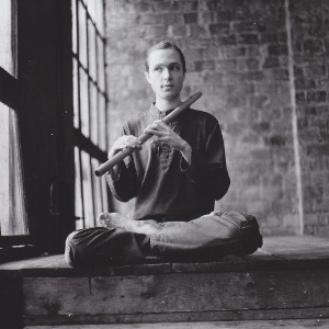Anton Kholomiov is a musician and programmer with a special interest in functional programming and indian classical music. He started learning music at the age of 14 with the acoustic guitar and later the piano and domra. More recently he has studied the Bansuri, a type of Indian wooden flute. He uses Csound on stage with the bands Kailash (https://soundcloud.com/kailash-project) and Sweet PAD (https://soundcloud.com/sweet_pad).

email: anton.kholomiov AT gmail.com