Introduction
This is the first in a series of articles in which I will explore interpretations of visual arts, stimuli, perception and cognition through sound and music. I shall be focussing on the use of Csound but many of the techniques and general concepts covered should be transferable to other audio tools. My intention is not to promote a methodical or slavish sonification of visual data, but instead to transfer a more advanced sense and understanding of the visual source onto sonic and musical materials. These interpretations may not always call out clearly to their visual cues but instead they may endeavour to find a representation of the visual-brain understanding of an artwork in an auditory-musical context.
I. Visual Conundrums
With the invention of photography in the 19th Century any remaining responsibility a painter might have felt to accurately represent his subject was effectively removed and the inclination to reinterpret and augment reality, where some form of representation was still present, became dominant. The understanding and rendering of perspective with mathematical rigour is seen as one of the great triumphs of the Renaissance, in particular in the art of Filippo Brunelleschi, but from the turn of the 20th Century it appeared to become increasingly imperative to jettison it. Some artists chose to flatten the 3-dimensionality of their subjects in order to remove the implied hierarchy that depth might suggest, others emboldened by the emerging science of cognitive psychology and with a better knowledge of the workings of the human brain sought to engage with the brain's process of analysing and understanding what the eyes see. Equipped with a mastery of rendering perspective, one can then pervert it. By far the most famous of these was the Dutch artist M.C. Escher. His work has always garnered interest from mathematicians and scientists and it is perhaps this interest that has tended to engender diminished regard from many mainstream art critics. Undeniable however is the intrigue that his work presents to the viewer.
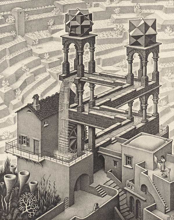
Figure 1. Waterfall (1961), M.C. Escher.
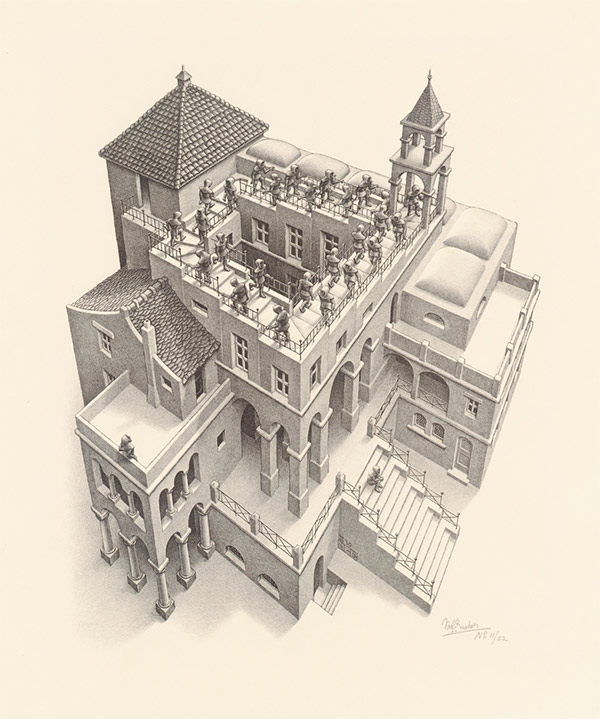
Figure 2. Ascending and Descending (1960), M.C. Escher.
The technique for which Escher is perhaps most famous is in his use of 'impossible' perspective. Waterfall [1] from 1961 explores our desire to understand a scene in terms of each element's location, high or low, near or far, and in terms of the incline of flat surfaces: rising or falling or completely horizontal. As if to emphasise the fact that incline is the subject here, Escher uses flowing water to inform us that a depicted channel is inclined slightly downhill. The punchline is to use a waterfall to confound the initial assertion of gravity by returning the water at the end of the channel back to its source - the body of water flows downward continually providing free and unlimited energy to a water wheel. Any true sense of movement is an illusion. Escher places his conundrum in mostly realistic surroundings to initially draw us in but also to camouflage the illusion. The scene is a Medieval town of high walls and narrow walkways. A figure stares up at the waterfall perhaps, like us, struggling to comprehend the paradox. Another figure, oblivious to the lunacy of the situation, hangs out washing. Impossibly sharp terracing stretches up and away in the background. Strange geometric shapes forming ornamental mouldings on top of the gazebos remind us that this is not reality.
Escher had employed the device of a central conundrum about which a scene is created earlier in Ascending and Descending [2] from 1960. This time two lines of monks ascend and descend a never ending staircase running along the top of a castle. The marching monks both draw our attention to the contradiction in the picture and drive home a sense of futility. Again Escher uses one figure staring perplexed up at the scene and another looking away from the scene to guide us both into and out of the scene. The sense of the uncanny is heightened by the masterly rendering of the perspective of the rest of the castle, viewed from an unusual position, high up in front of the castle—this contradictory staircase is not just an amateurish mistake.
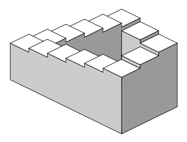
Figure 3. Penrose Steps (1959), Lionel and Roger Penrose.
Escher freely acknowledged precedence of the device used in Ascending and Descending to the 'Penrose Steps' [3] by Lionel and Roger Penrose. Lionel Penrose was a mathematician and psychiatrist and his son Roger was a mathematician who would later work with Stephen Hawking on research into black holes. Whilst the mechanics of the impossible staircase are essentially the same in the Penroses' version, the meaning and nuance is quite different. Escher imprints an artistic intention into his version through the use of the furniture and context within which he places his staircase. When transplanting analogous sonic techniques from proof of concepts into scenes of musical effectiveness, these auxiliary aspects of context and musical furniture are also critical.

Figure 4. Penrose Triangle (1958), Lionel and Roger Penrose.
The device used by Escher in Waterfall relates more closely to another Penrose invention: the 'Penrose Triangle' [4] or 'Impossible Triangle'. It had actually been discovered much earlier by the Swedish artist Oscar Reutersvärd but it appears that the Penroses' arrived at their version independently and they tend to be given more credit on account of having published their findings in The British Journal of Psychology [5] in 1958. Reutersvärd would go on to spend a lifetime exploring and discovering other examples of so-called 'impossible objects'. The essence of the illusion is that only two of the beams forming the triangle can confirm a possible orientation at any one time; the third always contradicts the other two. The shape either leans forward at 45 degrees, leans back or sits perpendicular but at 45 degrees to the plane of sight. Waterfall uses three Penrose triangles set edge to edge. The beams of the triangles are formed between the water channels and the gazebos.
It is not really possible to recreate any of these scenes or objects in reality. A form of representation is possible in sculpture but to experience it requires that we close one eye, only observe the piece from a specific location and that we don't attempt to walk around the object otherwise the trickery required will be revealed. These impositions essentially reduce 3d objects to two dimensions. Our experience when examining these impossible objects is of gaining understanding of individual elements: each joint, rod or plane makes sense on its own but when we attempt to draw back and understand the whole, we are confounded and are forced back in again to analyse each edge, corner and curve to try and find out where we went wrong. We find ourselves locked in a loop of understanding followed by confoundation. Experiencing these images we may be left feeling slightly unsatisfied and with a nagging sense of unease.
II. Sonic Interpretation
Selection of Appropriate Tools
Interpretation of these ideas and tricks will always be a struggle if we restrict ourselves to using the crude building blocks offered by mainstream music software. Quantisation—or at least coercion—of pitch and time into equally tempered notes and bars and beats will probably prove to be a hindrance. With its demand of complete precision and explication in defining even the simplest task, Csound represents the equivalent of the composer's (or sonic draughtsman's) pen, ruler and blank sheet of paper. It is no coincidence that some of the techniques discussed below emerged with the advent of computer music in the 1960s and 70s.
All of the examples in this article can be downloaded as a zip file containing Csound .csd files from here: FutileMovementExamples.zip
Shepard Tones, Risset Glissando
A well known and well documented interpretation of endless but ultimately futile movement in sound is 'Shepard Tones' [6], discovered by the psychologist Roger Shepard in 1964. Shepard uses the phenomenon of octave equivalence to mask the entry of a lower or higher tone above or below what we might perceive as the fundamental. Simply stated, octave equivalence is our inclination to perceive tones an octave apart as somehow 'the same'. Some people even struggle to correctly identify the higher or lower note when two tones an octave apart are played one after the other. Shepard tones present either a rising or falling scale. In the rising scale version (a descending scale version is equally valid), a tone one octave lower than the fundamental is faded in step by step in synchrony with the scalic steps so that when the fundamental reaches a point one octave above its starting location, the sub-octave, now at the original fundamental frequency, will attain the amplitude of the fundamental when at that frequency. Another way of looking at it is to consider partials whose amplitudes are wholly dependent upon a static spectral envelope or window. Once the sub-octave reaches the original frequency of the fundamental, it itself can now be regarded as a replacement fundamental (the octave above as its 1st harmonic overtone). Careful control of a partial's crossing over from a quiet irrelevance to a louder significance in how it is perceived is key. The entire process can be repeated but it is not a process defined by a beginning and an end, its shape is amorphous and all points along its progression can equally serve as beginnings or endings. Notions of fundamentals and overtones are nebulous and it is this characteristic that allows us to experience the duplicity of the Shepard Tones. The procedure can be expanded beyond two tones and beyond two octaves and in fact the success of the illusion will depend upon the choice of an appropriate range, number of partials and the shape of a spectral envelope that suitably de-emphasises the entry and exit of partials at the extremities of the texture. Our shift in focus from an upper partial to a partial one octave lower must be smooth, not abrupt, just as our reading of the continually rising Penrose staircase is smooth even once we realise that despite this, we have returned to where we started.
The tones climb upwards in relentless and identical steps, just like the monks in Ascending and Descending, but just like those monks, that rising is futile. The paradox hinges upon the expression of two contradicting ideas forced together. In Escher's version the ascending (or descending) stairs are forced to join through a distortion of perspective which the brain overlooks, in Shepard's tones the rising or falling chromatic movement is contradicted by a fixed spectral envelope which our brain similarly overlooks.
An innovation introduced by the French electronic music composer Jean-Claude Risset was to move from note to note continuously using glissando rather than through chromatic steps. If we were to interpret this visually, the Penrose staircase would become a helter-skelter. Risset first employed this effect in his 1968 piece Computer Suite from Little Boy (Part II: Fall). Using the technique, Risset represents the falling of the first atomic bomb (which had been nick-named 'Little Boy'). Risset has revisited the effect and with variations many times since. One of these variations is the harmonic arpeggio, a technique that has been explored in a previous Csound Journal article: Risset's Arpeggio - Composing Sound using Spectral Scans by Reginald Bain [15].
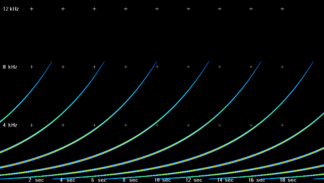
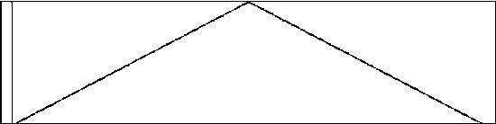
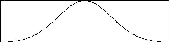
Figure 5. Spectrogram of a Risset Glissando (linear scale).
The spectrogram above depicts a Risset glissando that employs five partials. There are never more than five partials present at any one time. As one partial disappears at the upper frequency limit of the texture, its replacement appears at the bottom. The period of the texture, and lifespan of each partial, is 16 seconds.
Listening to the Risset glissando we are left with a similar feeling to that which we experience with Escher's Waterfall: futile movement. Instantly we realise we are moving somewhere but after some longer observation a sense that we might not be creeps in. Our initial notion is confounded, we are left feeling somewhat untethered and unsettled. In experiencing a visual artwork we create our own journey within it, we are free to ascend or descend the staircase, or to go upstream or downstream. Music cannot normally offer the listener a similar freedom, the composer must guide the listener either up or down a scale or glissando. There are interpretations of listener freedom possible however—when confronted with superimposed rising and falling textures the listener will tend to focus the ear on only one or the other at any one time.
Simplest Risset Glissando
A Risset glissando is very easy to create in Csound and there is an opcode that has the required mechanism effectively built-in. hsboscil generates a sound comprised of a stack of partials (we can choose the waveform but this is commonly a sinusoid) separated by octaves. These partials span out around a central frequency iBasFreq. The number of partials is prescribed using iOctCnt and the amplitude of each individual partial varies according to its pitch location between the maximum and minimum frequencies as shaped by the spectral envelope defined in the function table giOctFn. Its input argument kTone shifts all partials up one octave and it is this control that facilitates the endless glissando. We can cycle this control from 0 to 1 (the full range of the control) using a phasor (or from 1 to 0 by providing phasor with a frequency less than zero). It will not actually matter if this strays above 1 or less than zero as the effect will wrap around. The first example in the hsboscil page in the Canonical Csound Reference Manual [7] (example 374) demonstrates a Risset glissando. Below is another example:
; Example01.csd
<CsoundSynthesizer>
<CsOptions>
-odac -dm0
</CsOptions>
<CsInstruments>

0dbfs    =        1

giSine   ftgen    0,0,4097,10,1
giOctFn  ftgen    0,0,1024,-20,6,1,1 ; spectral envelope

alwayson 1

instr   1
 kAmp    =        0.2
 iOctCnt =        7     ; range of texture (in octaves)
 iBasFrq =        220   ; centre frequency
 kBrite  =        0     ; shift entire texture (in octaves)
 kTone   phasor   0.1   ; ramp waveform (range 0 - 1), frequency 0.1 hz.
 a1      hsboscil kAmp, kTone, kBrite, iBasFrq, giSine, giOctFn, iOctCnt
         out      a1
endin

</CsInstruments>
</CsoundSynthesizer>
The rate at which the texture rises is controlled by the frequency of the phasor. A negative frequency will result in a falling texture. Whether the effect is convincing will depend upon a number of factors: careful selection of the number of partials employed (iOctCnt) and the shape of the spectral envelope (giOctFn) are chief amongst these. It should be noted that poor quality speakers (such as laptop speakers) will add an additional spectral envelope which is likely to undermine the effectiveness of the illusion.
We will, for a moment, consider some of the options Csound provides for creating the spectral envelope. The nature of an appropriate window will depend upon the various settings chosen for the synthesis, in particular the number of partials, the base frequency and the rate of movement—experimentation is encouraged. Additional spectral shaping may be required to compensate for the ear's greater sensitivity to higher frequencies.
GEN07[8] can be used to generate a simple triangle shaped window:
giTriangle ftgen 0,0,1024,7,0,512,1,512,0
The first half of a sine wave, generated using GEN09[9], can be used to create a window that fades in and out more quickly:
giHalfSine ftgen 0,0,1024,9,0.5,1,0
An even more rapid fade in and fade out can be created using GEN16 [10]. In this example the values used to define the shapes of the two curves (-4 and 4) control the squareness of the window—the further away from zero these values are, the squarer the window becomes. If both values are zero the result is another triangle window:
giSquarish ftgen 0,0,1024,16,0,512,-4,1,512,4,0
Inverting the two values that defined the squareness of the window in the previous example will result in a 'pinched' window:
giPinched ftgen 0,0,1024,16,0,512,4,1,512,-4,0
GEN20[11] generates a number of preset windows, some of which offer further options for modification; 'Gaussian' is one of these. Its final parameter varies the breadth of the window. Values greater than 2 will result in a broader window (but also the possibility that partials will audibly and abruptly enter and exit in the Risset glissando) and values closer to zero will result in an increasingly narrow window:
giGaussian ftgen 0,0,1024,20,6,1,2
Even with the considerations discussed above, the trick is likely to be exposed if the speed of movement (phasor frequency) is excessive. Addition of some reverberation will help mask the joins, effectively what we are attempting here is sonic sleight of hand and any misdirection we can employ will help. If the addition of reverberation can be thought of as setting our sound in a real-world environment then this could be the equivalent of Escher decorating his Penrose staircases or triangles with windows, terraces or washing lines.
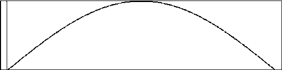
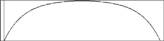
If we reduce the octave count to 2, increase centre frequency (iBasFrq) to 4000, and employ a spectral envelope that fades in and out much quicker, the spectrogram of the result looks like this:
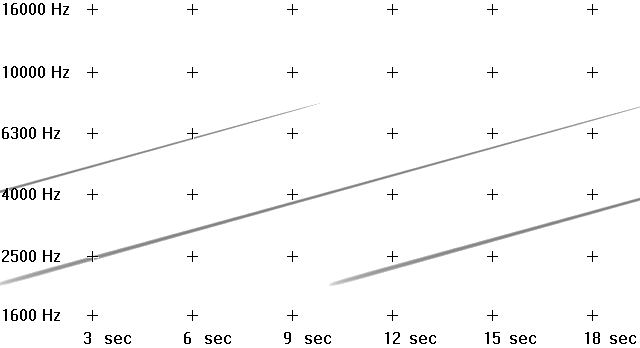
Figure 6. Spectrogram of a 2 partial Risset glissando (logarithmic scale).
This time the spectrogram employs a logarithmic scale so that parallel musical intervals will appear as parallel lines. We can see that there are never more that 2 octaves present and each partial is loudest at the central frequency. The entire structure covers a range of 3 octaves (2000 hz to 8000 hz).
Simplest Shepard Tones
Only a minor modification of our Risset glissando example using hsboscil is required to implement the chromatic scale of Shepard tones.
; Example02.csd
<CsoundSynthesizer>
<CsOptions>
-odac -dm0
</CsOptions>
<CsInstruments>

0dbfs    =        1

giSine   ftgen    0,0,4097,10,1
giOctFn  ftgen    0,0,1024,-20,6,1,1

instr    1
 aAmp    linsegr  0,0.01,1,0.01,0
 iOctCnt =        7
 iBasFrq =        220
 kBrite  =        0
 iTone   =        p4
 a1      hsboscil 0.2, iTone, kBrite, iBasFrq, giSine, giOctFn, iOctCnt
         out      a1*aAmp
endin

</CsInstruments>
<CsScore>
r 3
;----------tone
i 1 0 0.5 [0    ]
i 1 + 0.5 [1/12 ]
i 1 + 0.5 [2/12 ]
i 1 + 0.5 [3/12 ]
i 1 + 0.5 [4/12 ]
i 1 + 0.5 [5/12 ]
i 1 + 0.5 [6/12 ]
i 1 + 0.5 [7/12 ]
i 1 + 0.5 [8/12 ]
i 1 + 0.5 [9/12 ]
i 1 + 0.5 [10/12]
i 1 + 0.5 [11/12]
s
</CsScore>
</CsoundSynthesizer>
We only need to quantise kTone into 12 equal steps to create a chromatic scale. The score repeat r statement in conjunction with the end-of-section s statement are used to loop the scale three times.
Shepard Tones with Variations
Moving beyond the simple demonstration above, the following example uses rsplines[12] (random spline generators) to vary the speed (and direction if this value goes negative), the number of octave divisions and an additional parameter, gkBrite, which shifts the entire structure up or down.
; Example03.csd
<CsoundSynthesizer>
<CsOptions>
-odac -dm0
</CsOptions>
<CsInstruments>

0dbfs     =       1

giSine   ftgen    0,0,4097,10,1
giOctFn  ftgen    0,0,1024,16,0,512,-4,1,512,4,0

alwayson        1
alwayson        2

instr    1
 kTone   phasor   rspline:k(-4,4,0.05,0.2)     ; random speed and direction phasor
 kDiv    =        int(rspline:k(7,17,0.2,0.1)) ; random divisor (integer between 7 and 17)
 gkTone  =      int(kTone*kDiv)/kDiv
 if changed(gkTone)==1 then                    ; generate a new note when gkTone changes
  event "i",2,0,3600,gkTone
 endif
 gkBrite rspline  0,4,0.1,0.2                  ; randomly shift spectrum zero to +4 octaves
endin

instr    2
 if active:k(p1,0,1)>1 then                    ; turn off old note if a newer note exists
  turnoff
 endif
 aAmp    linsegr  0,0.01,1,0.01,0
 iOctCnt =        10
 iBasFrq =        110
 kBrite  =        0
 iTone   =        p4
 a1      hsboscil 0.6, iTone, gkBrite, iBasFrq, giSine, giOctFn, iOctCnt
         out      a1*aAmp
endin

</CsInstruments>
</CsoundSynthesizer>
The listener is guided up and down the 'staircase' at varying (and sometimes dizzying) speeds. The height of the 'steps' increase and decrease as we move and the entire 'staircase' is also rising and falling in space. The results are more interesting than before but as the speed of movement increases we can hear that the illusion is ruined. Whether this is a problem or not is a decision we must make as composers.
Risset Glissando from First Principles
The closed nature of an opcode—beyond its input arguments—inherently limits the possibilities for unique and further modification, it will therefore prove beneficial to implement the technique from first principles. Coincident layers of oscillators will be required to create the partials. Hard coding these layers is not ideal as adding or removing layers later on will prove cumbersome. A better approach is to use a recursive UDO. This is a technique that was described by Steven Yi in the summer 2006 edition of the Csound Journal in his article "Control Flow - Part II"[13]. With this implementation we can now go beyond hsboscil's partial limits of between 2 and 10 and we can also employ partial separations other than an octave through the use of the kIntvl parameter. This is defined in semitones and can be modulated at k-rate resulting in warping of the spectrum. Partial gaps other than an octave or a factor of an octave will remove the enhancement provided by octave similarity but again this is an informed choice available to us as composers. A variety of possibilities are explored through the five score events in the following example:
; Example04.csd
<CsoundSynthesizer>
<CsOptions>
-odac -dm0
</CsOptions>
<CsInstruments>
0dbfs     =            1

giWfm    ftgen        0,0,4097,10,1        ; audio waveform: a sine wave
giAmpFn  ftgen        0,0,1024,-20,6,1,1.2 ; gaussian window

opcode EndlessGlissSynth,a,kkkiiiip
 kPhase,kCentre,kIntvl,iAmpFn,iWfm,iRndPhs,iLayers,iCount  xin

; calculate phase for this layer (and wrap within the range 0 to 1)
 kLPhs    wrap         kPhase+((iCount-1)/iLayers),0,1

; read amplitude from spectral envelope
 kAmp     tablei       kLPhs,iAmpFn,1

; complete texture range (in semitones)
 kRange   =            iLayers * kIntvl

; calculate note (number)
 kNote    limit        kCentre - (kRange*0.5) + (kRange * kLPhs),0,127

; amplitude scaling. (attenuate higher notes)
 kAmpScl  scale        logcurve:k(kNote/127,4),0.01,1
 a1       poscil       kAmp*kAmpScl,cpsmidinn(kNote),iWfm ,rnd(iRndPhs)
 if iCount<iLayers then                        ; call next layer (if required)
  amix EndlessGlissSynth kPhase,kCentre,kIntvl,iAmpFn,iWfm,iRndPhs,iLayers,iCount+1
 endif
          xout         a1 + amix              ; return audio to caller instrument
endop

instr   1
 kAmp     =            p4
 iLayers  =            p5    ; number of layers
 kIntvl   init         p6    ; gap between adjacent layers
 kCentre  init         p7    ; central pitch as a note number
 kPhase   phasor       p8/iLayers
 iRndPhs  =            p9    ; random initial phase amount
 aMix     EndlessGlissSynth kPhase,kCentre,kIntvl,giAmpFn,giWfm,iRndPhs,iLayers
 aEnv     linsegr      0,0.01,1,0.01,0
          out          aMix * kAmp * aEnv
endin

<CsScore>
;----------amp--layers--intvl--centre--rate--RndPhs
i 1 0  14  0.7     6      12    60     0.15    0
i 1 15 14  0.2    40       3    60     0.2     0
i 1 30 14  0.2    40     0.5    72     2       0
i 1 45 14  0.2    40     0.5    72     2       1
i 1 60 29  0.07  112       2    60     -0.3    1
</CsScore>

</CsInstruments>
</CsoundSynthesizer>
If the interval that separates partials is very small—less than a semitone—it becomes harder to distinguish the movement of partials. Instead we start to hear sidebands produced by the beating between the closely tuned oscillators. The emphasis of this effect when using more than two partials is dependent upon the mathematical correlations between their phases. This correlation can be upset by randomising their starting phases. An input argument of the UDO, iRndPhs, is provided for doing this.
Risset Glissando as a Signal Processor
There is no reason why we should restrict ourselves to using the critical data used by each partial—amplitude and frequency—with sine wave oscillators. Beyond modifying the oscillator waveform or using other more specialised sound generators, we can use this data with sound modifiers such as filters. The following example replaces the poscil oscillator with a flanger opcode to create a comb filtering effect. The UDO is modified to receive an input audio signal and to return an output audio signal: a mix of all transformed layers. The input signal in this example is a generic crackling sound.
; Example05.csd
<CsoundSynthesizer>
<CsOptions>
-odac -dm0
</CsOptions>
<CsInstruments>

0dbfs      =         1

giAmpFn    ftgen     0,0,1024,7,0,512,1,512,0 ; triangle

opcode EndlessGlissComb,a,akkkiip
 aSig,kPhase,kCentre,kIntvl,iAmpFn,iLayers,iCount  xin
 kLPhs     wrap      kPhase+((iCount-1)/iLayers),0,1     ; layer phase position
 kAmp      tablei    kLPhs,iAmpFn,1         ; read amplitude from spectral envelope
 kRange   =            iLayers * kIntvl                 ; total range (semitones)
 kNote    limit        kCentre-(kRange*0.5)+(kRange*kLPhs),0,127 ; calc. note num.

 adel      interp    1/cpsmidinn(kNote)                  ; pitch to delay time
 aRes      flanger   aSig, adel, 0.999                   ; comb filter (flanger)
 aRes      dcblock2  aRes                                ; remove DC offset

 if iCount<iLayers then                           ; create next layer (if required)
  aMix EndlessGlissComb aSig,kPhase,kCentre,kIntvl,iAmpFn,iLayers,iCount+1
 endif
           xout      (aRes*kAmp) + aMix     ; return all audio to caller instrument
endop

instr   1
 kAmp      =         0.2
 iLayers   =         24                               ; number of layers
 kIntvl    init      3                                ; gap between adjacent layers
 kCentre   init      60                               ; central pitch as a note number
 kPhase    phasor    -0.05/iLayers

 ; generate some audio
 aSig      dust2     0.5,10                           ; generate some  audio dust
 aSig      butlp     aSig,cpsoct(randomi:k(6,12,8,1)) ; random LP filtering

 aMix      EndlessGlissComb  aSig,kPhase,kCentre,kIntvl,giAmpFn,iLayers
           out       aMix
endin


<CsScore>
i 1 0 300
</CsScore>

</CsInstruments>
</CsoundSynthesizer>
The input sound employed here is rather uninteresting but with more recognisable source material the result can be more interesting and the listener is distracted from the application of the illusion in a shift that mirrors the move from the Penroses' dislocated staircase to Escher's surreal monastery. This is also one example of how a sonic implementation could move from scientific demonstration to artistic edifice.
Further experimentation could involve the technique described above but with any of the other filters and signal processors contained within Csound's armoury—our raw input is simply streams of frequency and amplitude data. This approach suggests an advantage over traditional LFO modulated DSP effects, which can sometimes sound 'trapped' as they 'bounce' off the maxima and minima of their LFO waveforms.
Shepard Tones as Real-time Csound Events
Other possibilities are available if we use the amplitude and frequency data that we originally used with oscillators as p-field values that we send as bundles in Csound note events. In the following example, Csound events are generated within the UDO using the event opcode. It is triggered periodically by a metronome (metro opcode). In this example the sound producing instrument is a plucked string-like sound created using the wguide1 opcode, but it could generate sound using practically any other means and still express the same general effect. It is only required that p4 and p5 are used for pitch (note number) and amplitude respectively. Bear in mind that instrument 3 is being triggered multiple times upon each new step of the scale, once for each layer, so considerable polyphony can be demanded of instrument 3. A number of other options, some that have already been employed in previous examples, are implemented: step size can be any value and is not restricted to single semitones, the interval between adjacent partials need not be octaves and the scheduling of coincident partials can be smeared by some random time value (iRndWhen) or by arpeggiation (iArp). The four score events in this example demonstrate these options.
; Example06.csd
<CsoundSynthesizer>
<CsOptions>
-odac -dm0
</CsOptions>
<CsInstruments>

0dbfs      =         1

giAmpFn    ftgen     0,0,1024,7,0,512,1,512,0

opcode  EndlessScale,0,kkkkkkkiiip
 kRate,kCentre,kStep,kIntvl,kDur,kRndWhen,kArp,iInsNum,iAmpFn,iLayers,iCount        xin
 ktrig     metro     kRate

 kRange    =         iLayers * kIntvl                     ; range of entire texture
 kBase     =         kCentre - (int(iLayers/2) * kIntvl)  ; lowest note (number)
 kNote     init      i(kBase) + ((iCount-1)*i(kIntvl))    ; initial note

 if ktrig==1 then
  kAmp     table     (kNote-kBase)/(iLayers*kIntvl),iAmpFn,1 ; amp. from spec. env.
           event "i",iInsNum,rnd(kRndWhen)+((iCount-1)*kArp),kDur,kNote,kAmp,iCount
  kNote    wrap      kNote+kStep,kBase,kBase+(iLayers*kIntvl) ; increment note
 endif

 if iCount<iLayers then  ; call next layer (if required)
           EndlessScale kRate,kCentre,kStep,kIntvl,kDur,kRndWhen, \
                        kArp,iInsNum,iAmpFn,iLayers,iCount+1
 endif

endop

instr      1
 kRate     =         p4      ; rate of notes (per second)
 ktrig     metro     kRate
 kCentre   init      p5      ; centre note (note number)
 kStep     init      p6      ; step size (semitones)
 kIntvl    init      p7      ; interval between layers
 iLayers   init      p8      ; number of layers
 iInsNum   =         3       ; instrument number of instr to play a sound
 kDur      =         3/kRate ; note duration
 kRndWhen  =         p9      ; range of random note start time
 kArp      =         p10     ; arpeggiation time
           EndlessScale kRate,kCentre,kStep,kIntvl,kDur,kRndWhen,kArp,iInsNum,giAmpFn,iLayers
endin

instr      3 ; a pluck sound
 icps      =         cpsmidinn(p4)
 iamp      =         p5
 aenv      expsegr           1,0.1,0.001
 aImpEnv   expseg    0.0001,0.001,1,10/icps,0.0001,1,0.0001
 axcite    butlp     pinkish:a(aImpEnv*iamp),limit:i(icps*2,0,sr/2)
 a1        wguide1   axcite,icps,limit:i(icps*16,0,sr/2),0.999
 a1        dcblock2  a1
           outs      a1*aenv,a1*aenv
endin


<CsScore>
;-----------p4-----p5-----p6-----p7-----p8------p9------p10
;----------rate--centre--step--intvl--layers--RndWhen--Arp
i 1 0  14   2      60     1     12       8       0       0
i 1 15 14   2      60    0.5    12       8       0       0
i 1 30 14   4      48     2      5      12       0     [1/3]
i 1 47 14   3      36    -1      7      12     0.1       0
</CsScore>

</CsInstruments>
</CsoundSynthesizer>
Notice that instrument 3 is also sent the layer number of the layer that generated it as p6. In this example it is an unused p-field but it could be used as an index to define some unique layer dependent transformation (Example08.csd makes use of this option).
This is another example of an implementation that becomes more colouristic and artistic than scientific. One aspect of note is that wguide1's tuning anomalies, particularly noticeable as notes get higher, will undermine successful employment of octave similarity in the illusion, although tuning correction could be used to counteract this discrepancy.
Shepard Tones as a MIDI Instrument
With some modifications we can adapt the instrument from the previous example for use with a MIDI keyboard. Giving the performer this control will be a good way to explore less predictable movement from note to note. As expected, moving up the keyboard will not result in continually higher and higher notes but instead an exhibition of cyclical spectral recurrence with a cycle period depending on the values provided for iIntvl (interval between layers in semitones) and iStepSize (size of the interval between adjacent notes in semitones). There will be cyclical recurrence every iStepSize * iIntvl notes. In the example below, given the values for these two parameters (iStepSize=0.5, iIntvl=7) this recurrence will be every 14 notes. A variable created within the UDO, iStep, divides each cycle into the required number of steps. So in the example, iStep will loop through the values 0, 0.5, 1, 1.5 ... 6.5, 0 as we progress up the keyboard chromatically.
; Example07.csd
<CsoundSynthesizer>
<CsOptions>
-odac -dm0 -Ma
</CsOptions>
<CsInstruments>

0dbfs      =         1

giAmpFn    ftgen     0,0,1024,7,0,512,1,512,0

opcode  EndlessScaleMIDI,a,iiiiiiiip
 iNoteNum,iStepSize,iCentre,iVel,iLayers,iIntvl,iInsNum,iAmpFn,iCount    xin
 iStep     =         (iNoteNum*iStepSize)%iIntvl           ; wrapped step value
 iRange    =         iLayers * iIntvl                      ; entire range
 iBase     =         iCentre - (int(iLayers/2) * iIntvl)   ; lowest note

; note (number) for this layer
iNote     wrap      iBase+((iCount-1)*iIntvl)+iStep, iBase, iBase+(iLayers*iIntvl)

 iAmp     table      (iNote-iBase)/(iLayers*iIntvl),iAmpFn,1
 aSig     subinstr   iInsNum,iNote,iAmp*iVel,iCount
 if iCount<iLayers then
  aMix    EndlessScaleMIDI  iNoteNum,iStepSize,iCentre,iVel,\
                            iLayers,iIntvl,iInsNum,iAmpFn,iCount+1
 endif
          xout       aSig + aMix
endop

instr      1
 iNoteNum  notnum            ; MIDI note number
 iStepSize =         0.5     ; step size from note to note
 iIntvl    =         7       ; interval between layers
 iCentre   =         36      ; centre note (note number)
 iVel      veloc     0,1     ; MIDI note velocity
 iLayers   =         12      ; number of layers
 iInsNum   =         3       ; instrument number of instr to play a sound
 aMix      EndlessScaleMIDI iNoteNum,iStepSize,iCentre,iVel,\
                            iLayers,iIntvl,iInsNum,giAmpFn
 aEnv      expsegr   1,0.1,0.001 ; anti click envelope
           out       aMix*aEnv
endin

instr      3 ; a pluck sound
 icps      =         cpsmidinn(p4)
 iAmp      =         p5
 aImpEnv   expseg    0.0001,0.001,1,10/icps,0.0001,1,0.0001
 axcite    butlp     pinkish:a(aImpEnv*iAmp),limit:i(icps*2,0,sr/2)
 aSig      wguide1   axcite,icps,limit:i(icps*16,0,sr/2),0.999
 aSig      dcblock2  aSig
           out       aSig
endin

</CsInstruments>
</CsoundSynthesizer>
No MP3 rendering is provided as this example needs live performance from a MIDI keyboard.
As we form melodic passages using this instrument, the sense of whether intervals are rising or falling can become ambiguous, particularly if larger steps are employed. For the player, an unbiased judgment of what is perceived is more difficult on account of an awareness of the physical movement over the keys, but for the listener, the sense of whether a phrase is rising or falling is governed more by the Gestalt principle of continuation. If we play a rising phrase C-E-G then we tend to perceive this as rising, but if we omit the E, then the notes C to G can be perceived as either rising or falling. This phenomenon of ambiguity is similar to that encountered with the 'Necker' cube which can be perceived either as being observed from above or from below at different times.

Figure 7. Necker Cube[14].
Endless Speed Change
In the conglomerate tones we have created so far we have been dealing with stacks of partials separated by equal musical intervals. If we scale these pitches down dramatically they can become rates of pulsation rather than pitches—not a change of type but of scale. We might also switch from using note numbers and intervals in semitones to using frequencies and frequency ratios as units of measurement. Rather than creating illusions of 'endless' pitch movement we shall be implementing 'endless' tempo change.
The following example builds upon Example04.csd in which we implemented a Risset glissando from first principles. This time the pitch (frequency) is used to drive metronomes which in turn trigger note event generation using the schedkwhen opcode. Now when we hear the superimposition of different layers, we perceive subdivisions of a pulse. If kDiv (beat subdivision) is 2, then the 2nd layer from the bottom pulses twice as fast as the first, the 3rd layer pulses four times as fast as the first and so on. If we restrict ourselves to integers or simple fractions such as 3/2 for kDiv, then synchronicity will occur periodically between layers and pulse divisions should be evident to the listener. If we use more complex fractions for kDiv then the result will be less coherent. In this example the layer numbers are sent to the sound producing instrument (instr 3) as p5 and this is used to give each layer a unique pitch. This makes the result more interesting to listen to but draws it further away from the idea of creating any sort of illusion. No one will hear this as an endless speed change, the mechanism is clearly evident.
A polyphony control mechanism is implement that can restrict polyphony within a layer when metronome clicks are extremely fast. This is activated by defining a negative duration value for kDur in instrument 1. In this mode if kDur is ever longer than the gap to the next note event in that layer then it will be truncated to whatever that gap time is. (Gap time is always 1/metronome rate.)
; Example08.csd
<CsoundSynthesizer>
<CsOptions>
-odac -dm0
</CsOptions>
<CsInstruments>
0dbfs     =         1

giAmpFn  ftgen 0,0,1024,7,0,512,1,512,0 ; triangle

opcode  EndlessSpeedChange,0,kkkkkiip
 kInsNum,kDur,kPhase,kCentre,kDiv,iAmpFn,iLayers,iCount  xin
 kLPhs      wrap     kPhase+((iCount-1)/iLayers),0,1 ; local phase
 kAmp       tablei   kLPhs,iAmpFn,1                  ; read amp. from envelope
 kRate      scale    kLPhs,iLayers/2,-iLayers/2      ; rate function (in octaves)
 kRate      =        kCentre * (kDiv ^ kRate)        ; rate (hz)
 kTrig      metro    kRate                           ; trigger for this layer

  if kDur<=0 then                  ; branch to duration control if negative value
   kDur2            limit       abs(kDur),0.1,1/kRate ; limit to time gap (1/kRate)
  else
   kDur2            =           kDur                ; otherwise just use kDur value
  endif

          schedkwhen  kTrig,0,0,kInsNum,0,kDur2,kAmp,iCount
 if iCount<iLayers then                              ; call next layer if required
     EndlessSpeedChange kInsNum,kDur,kPhase,kCentre,kDiv,iAmpFn,iLayers,iCount+1
 endif
endop

instr      1 ; define texture values and call UDO
 kAmp      =         0.2
 kInsNum   init      3       ; number of sound producing instrument
 kDur      init      -1.3    ; negative duration activates duration control
 iLayers   =         4       ; number of layers
 kDiv      init      2       ; beat division
 kCentre   init      4       ; centre frequency (rate)
 kPhase    phasor    -0.1    ; phase position through entire pattern
           EndlessSpeedChange  kInsNum,kDur,kPhase,kCentre,kDiv,giAmpFn,iLayers
endin

instr      3 ; sound producing instrument
 iLayer    =         p5
 iNote     =         48 + (iLayer * 5)
 iDur      =         0.9*(1+(((64-iNote)/127)*3))
 iVel      =         p4^3
 aEnv1     expsegr   1,     iDur,0.0001,0.01,0.0001
 aEnv2     expsegr   1,0.2* iDur,0.0001,0.01,0.0001
 aEnv3     expsegr   1,0.02*iDur,0.0001,0.01,0.0001
 aPart1    oscili    (aEnv1-0.0001) * 1   , cpsmidinn(iNote)
 aPart2    oscili    (aEnv2-0.0001) * iVel, cpsmidinn(iNote) * 3.37
 aMod      oscili    aEnv3,cpsmidinn(iNote) * 2.77
 aMix      sum       (aPart1+aPart2)*iVel*0.3*(1-(aMod*iVel))
           out       aMix
endin

<CsScore>
i 1 0 3600
</CsScore>
</CsInstruments>
</CsoundSynthesizer>
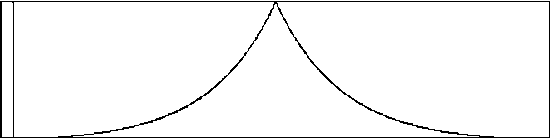
We can illustrate the mechanism at work further using the spectrogram below which depicts a 2 layer texture with a frequency ratio of 4. The phase relationship of 180 degrees between the two layers is evident as they fade in and out and the constant pulse ratio of 4:1 is also confirmed.
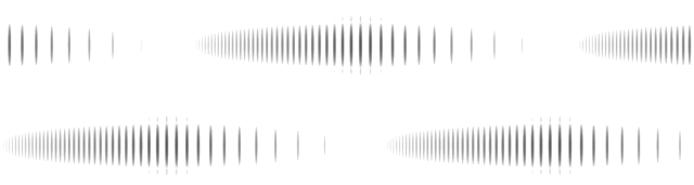
Figure 8. Two voice endless speed change.
The example presented here is very simple and there is obvious scope for increased layering and complexity of relationships between the different layers. It will become clear however that the threshold between rhythmic complexity and rhythmic chaos is a fine one. Our ability to unscramble rhythmic polyphony is weaker than our ability to make sense of a polyphony of pitches. The rhythmic texture's purpose remains clear as long as we are still able to discern sustained internal motivic transformation, once we lose this, the texture can become an amorphous cloud.
III. Musical Interpretation and Further Consideration
How these techniques are used musically requires careful consideration. Uses that flaunt their trickery may succeed only at the level of novelty. If the only real interest is the device itself then the music is unlikely to survive deeper scrutiny. Escher situates his visual sleights of hand in realistic environments with additional buildings, people and trees. In Waterfall, the three Penrose triangles are expertly folded within the elements from which they are formed: the pillars and water channels, this approach staves off our recognition of the trickery. Once it is discovered we are left with a vaguely dizzying confusion and a sustained intrigue. Clearly another aspect of Escher's work that elevates the concept beyond that of a graphical demonstration is the degree of expert craft employed in its execution. Demonstrations of many of the sonic techniques introduced in this article are easy to find on the Internet on YouTube, but it is harder to find any that are not just garish or have any evolved musical deployment.
The examples I have presented here are necessarily basic in order to clearly demonstrate the techniques introduced. Enormous scope exists for much greater manipulation; these examples are not finished articles, just raw materials. I have tended to define many of the critical values as static rounded integers to provide clear starting points. Experiments should be undertaken to explore the effects of non-integer values and to modulate these during note performance (k-rate) in interesting ways. Some of the examples exhibit a cyclical stasis; this is something that is difficult to sustain in music and its dramatic value is doubtful, certainly in the longterm. Furthermore, sensory instructions that confound our senses tend to leave us unsettled so we must consider what our musical aim is and what the consequences of our choices are. Drawing inspiration from visual sources for sonic investigation is only a beginning and interpretation can and should go beyond a responsibility to point towards its source. The profound difference between the cognitive mechanisms of our visual and aural senses will also demand that we develop any work in response to the functioning of our musical sense.
References
[1] M.C. Escher, Waterfall (1961). [Online] Available: http://www.mcescher.com/gallery/impossible-constructions/waterfall/ [accessed July 7, 2015].
[2] M.C. Escher, Ascending and Descending (1960). [Online] Available: http://www.mcescher.com/gallery/impossible-constructions/ascending-and-descending/ [accessed July 7, 2015].
[3] Lionel and Roger Penrose, Penrose Stairs (1958), Design: Lionel and Roger Penrose. [Online] Available: https://en.wikipedia.org/wiki/Penrose_stairs [accessed July 7, 2015].
[4] Lionel and Roger Penrose, Penrose Triangle (1959), Design: Lionel and Roger Penrose. [Online] Available: https://commons.wikimedia.org/wiki/File:Penrose-dreieck.svg#/media/File:Penrose-dreieck.svg [accessed July 10, 2015].
[5] Penrose, L. S., and Penrose, R. "Impossible objects: A special type of visual illusion," British Journal of Psychology 49(1) : 31-3 (1958).
[6] Roger N. Shepard. "Circularity in Judgements of Relative Pitch," Acoustical Society of America 36, 3005 (December, 1964).
[7] Barry Vercoe et Al. (2005). "hsboscil," The Canonical Csound Reference Manual. [Online] Available: http://csound.github.io/docs/manual/hsboscil.html [accessed July 6, 2015].
[8] Barry Vercoe et Al. (2005). "GEN07," The Canonical Csound Reference Manual. [Online] Available: http://csound.github.io/docs/manual/GEN07.html [accessed July 6, 2015].
[9] Barry Vercoe et Al. (2005). "GEN09," The Canonical Csound Reference Manual. [Online] Available: http://csound.github.io/docs/manual/GEN09.html [accessed July 6, 2015].
[10] Barry Vercoe et Al. (2005). "GEN16," The Canonical Csound Reference Manual. [Online] Available: http://csound.github.io/docs/manual/GEN16.html [accessed July 6, 2015].
[11] Barry Vercoe et Al. (2005). "GEN20," The Canonical Csound Reference Manual. [Online] Available: http://csound.github.io/docs/manual/GEN20.html [accessed July 6, 2015].
[12] Barry Vercoe et Al. (2005). "rspline," The Canonical Csound Reference Manual. [Online] Available: http://csound.github.io/docs/manual/rspline.html [accessed July 6, 2015].
[13] Steven Yi. (2006). "Control Flow Part 2," Csound Journal [Online], Volume 1 Issue 4, Summer 2006. Available: http://csoundjournal.com/2006summer/controlFlow_part2.html [accessed July 10, 2015].
[14] BenFrantzDale. Necker Cube (uploaded 2007). [Online] Available: https://commons.wikimedia.org/wiki/File:Necker_cube.svg#/media/File:Necker_cube.svg [accessed July 10, 2015].
[15]Reginald Bain. (2015). "Risset's Arpeggio - Composing Sound using Spectral Scans," [Online] Available: http://csoundjournal.com/issue17/bain_risset_arpeggio.html [accessed April 26th, 2015].